A common experimental method used for AB testing is Null hypothesis-based statistical testing (NHST). In the NHST approach, the scientist collects data from some process or group of interest, then performs a statistical test to evaluate whether the distribution of collected samples is statistically different from the distribution generated by some baseline–aka “Null”–process or control group.
Due to inherent randomness in the world and the fact that sampling procedures will always be imperfect, it is possible that the researcher detects a statistically significant difference when, in fact, there isn’t one. This scenario is called a False Positive or Type I Error, and each NHST has its own acceptable Type I Error rate. The acceptable False Positive rate is generally referred to as \(\alpha\), and tends to be set in the range of \(1 \%-5 \%\).
A key step when using NHST is to establish a minimum number of samples \(N\) to collect in order to provide statistical guarantees on the expected False Positive rate. This procedure is know as power analysis.
Sometimes, during the data collection process, the scientist will “peek” at the data prematurely, before data collection has reached the \(N\) samples prescribed by power analysis. The scientist will then perform preliminary analyses and statistical tests on this incomplete dataset. This is where the p-hacking begins!
Say the scientist finds no statistical difference from the Null hypothesis. In this case, it highly likely that the scientist will collect more data in order to try to further establish whetehr there is a real difference. However, if a difference is detected, data collection is likely to be stopped–a form of confirmation bias, if you will. This strategy of peeking and conditionally continuing data collection based on test results obtained from the partial dataset invalidates the assumptions of the statistical test and inflates the likelihood of observing a false positive.
Below we use simulation to demonstrate the degree to which various data peeking strategies can inflate the False Positive rate of the statistical procedure, and compare those False Positive rates to a valid, no-peeking analysis strategy.
In each of 5,000 simulations below we generate a scenario where our data are sampled from a distribution that has zero mean–in this case a standard Normal. We then use a one-sample t-test to infer whether or not the mean of those samples differs signficantly from zero (the Null hypothesis). Since the samples do in fact have zero mean, we intuitively would expect to always detect no difference from zero. However, due to randomness in the sampling process, we’ll obtain a difference by chance some small percentage of the time.
Additionally, for each simulation we’ll “peek” at the partial dataset at various points during the data collection, based one of the following peeking strategies:
After each peek at the current dataset, we then decide whether to keep collecting data contingent on what we’ve observed so far:
Given that we know the ground truth distribution, we can calculate how much the False Positive rate has increased for each peeking strategy over the course of data collection.
The results of the simulation are plotted in Figure 1.
Figure 1, False positive (Type I) error rates associated with various data-peeking strategies. As we increase the frequency of data peeking, we increase the False Positive rate of our inference procedure. This inflation increases with the number peeks and samples collected. If we were to peak at every sample, we would have a nearly 1 in 2 chance of a False Positive after collecting ~500 samples. No data peeking closely follows the researcher-defined accptable False Positive rate for the experiment \(\alpha=0.05\).
import numpy as np
from scipy import stats
from matplotlib import pyplot as plt
from vis import COLORS, save_figure
np.random.seed(123)
"""
Simulate 5000 experiments with 500 samples each. There is no statistical
difference in the mean of the sampled data from zero (our Null Hypothesis)
"""
n_samples_per_simulation, n_simulations = 500, 5000
real_mean = 0
sampling_distribution = stats.norm(loc=real_mean)
simulations = sampling_distribution.rvs(
size=(n_samples_per_simulation, n_simulations)
)
# Simulate many hypothesis tests, increasing the sample size for each
p_values = []
n_samples = []
min_samples = 3 # Minimum samples used to run a t-test
for n_samples_used in range(min_samples, n_samples_per_simulation):
n_samples.append(n_samples_used)
# p-values obtained from one-sample t-test
p_values.append(
stats.ttest_1samp(simulations[:n_samples_used], 0., axis=0).pvalue
)
# Make null-hypothesis decisions based on p-values
alpha = .05 # Researcher-defined acceptable Type I error rate
decisions = np.array(p_values) <= alpha
"""
We simulate peeking by denoting all observations that follow
observing an initial positive result to also be considered positive.
This is equivalent to not collecting any more data.
"""
# Simulate peeking every N-th sample strategy
peeking_strategy = [1, 10, 20, 50]
peeking_strategy_colors = [
"black",
COLORS.dark_red,
COLORS.red,
COLORS.salmon
]
plt.subplots(figsize=(8, 8))
for ci, peek_every_nth in enumerate(peeking_strategy):
intermitten_peeking_decisions = decisions[::peek_every_nth].cumsum(axis=0) >=1
intermitten_peeking_type_I_error_rate = intermitten_peeking_decisions.mean(axis=1)
# Add plot for this strategy
label = 'Every Sample' if peek_every_nth == 1 \
else f'Every {peek_every_nth}th Sample'
plt.plot(
n_samples[::peek_every_nth],
intermitten_peeking_type_I_error_rate,
color=peeking_strategy_colors[ci],
label=label
)
"""
We simulate no peaking as just the average Type I error
rate across all simulations without any results-dependent
screening.
"""
type_I_error_rate = decisions.mean(axis=1)
plt.plot(n_samples, type_I_error_rate, color=COLORS.blue, label='No Peeking')
plt.axhline(
alpha,
color=COLORS.gray,
linestyle='--',
label=r'$\alpha={:0.2f}$'.format(alpha)
)
plt.ylim(0, .6)
plt.xlim(min_samples, n_samples_per_simulation - peeking_strategy[-1])
plt.xlabel("Number of Samples")
plt.ylabel("Type I Error Rate")
plt.title(
"The effect of peeking at your AB test\n"
"results before data collection is complete"
)
plt.legend(title="Peeking Strategy")
plt.grid();
We can see that the more often we peek at our data, the larger our False Positive rate becomes over the course of the experiment’s data collection. In the worst case scenario, where we peek at every sample, our False Positive rate is nearly 50% after collecting ~500 samples!
We can also see how not peeking allows us to maintain the guarantees of the statistical test on False Positive rate. When we don’t peek at our data, our expected Type I error rate is consistent with the \(\alpha\) used in the t-test.
Data-peeking is just one of many spooky gotchas that come along with using Null hypothesis-based statistical tests (NHST). This particular p-hacking effect comes up when we prematurely run statistical tests on our experiment data before the required dataset size has been reached. If you’ve ever said something like “let’s just take a look at the experimet to see if we’ve reached statsig,” then you’re probably p-hacking!
The negative affects of data-peeking can be minimized by sticking to standardized protocols for running experiments that use NHSTs: running an initial power analysis to calculate the required sample size for a desired effect size and statistical power, then holding off your statistical analysis till the proper sample size has been reached.
A well-behaved statistical test should provide uniformly-distributed p-values. This is because the test shouldn’t favor any one portion of the hypothesis space over the others. This is demonstrated in Figure 1, which plots the distribution of p-values that result from running two-sample t-tests on 10,000 simulated datasets (\(N=10\)) having no difference between the two samples being tested, i.e. the Null Hypothesis \(H_0=\text{True}\).
Figure 1, p-values from a well-behaved statistical test. p-values should be uniformly distributed; here we choose twenty equally-sized bins, corresponding with \(\alpha=0.05\). Even when there is no effect, i.e. \(H_0=\text{True}\), 5% of trials will indicate a “significant” effect by chance (red). Additionally, 5% of trials will be “So close” to showing significance (blue). N chasing is often performed on these “So close” trials by collecting additional data points.
import numpy as np
from scipy import stats
from abra.vis import Gaussian, COLORS # requires abracadabra
from matplotlib.patches import Rectangle
# Simulate multiple experimental datasets where H_0=True
# run t-tests, then collect the resulting p-values
ALPHA = 0.05
n_obs_per_trial, n_trials = 10, 10000
np.random.seed(1234)
null = Gaussian()
datasets = null.sample((2, n_obs_per_trial, n_trials))
pvals = stats.ttest_ind(datasets[0], datasets[1], axis=0).pvalue
def pval_rate_histogram(pvals, resolution=ALPHA, color='white', label=None):
"""Util for plotting the number of p-values that occur within buckets
of size `resolution`.
"""
bins = np.arange(0, 1, resolution)
factor = 1 / float(len(pvals))
cnts, bins = np.histogram(pvals, bins=bins)
return plt.hist(bins[:-1], bins, weights=factor*cnts, color=color, label=label, edgecolor='black')
# Plot distribution of non-hacked p-values
plt.subplots(figsize=(10, 6))
cnt, bin_left, patches = pval_rate_histogram(pvals, color=COLORS.light_gray, label='p-values')
plt.ylim([0, .07])
# Highlight the trials bucket associated with false positives as
# well as those trials that are "Soo close" to being "significant"
## False positives trials
expected_type_I = patches[0]
expected_type_I.set_color(COLORS.red)
expected_type_I_rate = cnt[0] * 100.
expected_type_I.set_label(f"{round(expected_type_I_rate)}% of Trials are False Positives")
## So close to being "significant" trials
near_type_I = patches[1]
near_type_I.set_color(COLORS.blue)
near_type_I.set_label("'Soo close!' Trials")
plt.axhline(ALPHA, color=COLORS.dark_red, label='Expected Type I Error Rate')
plt.xlabel('p-values')
plt.ylabel('Proportion of Trials')
plt.title("p-values from a well-behaved statistical test are uniform")
plt.legend()
Because the p-vlaues are uniformly distributed, if you histogram the p-values into 20 equally-sized bins, you would expect each bin to be associated with roughly 5% of trials. Consequently, we would expect a default false positive rate \(\alpha\) of 0.05. It turns out this resolution of p-value breakdown that is a pretty common scientific standard and is one of the reasons everyone uses an \(\alpha=0.05\) in hypothesis tests.
Figure 1 also highlights in blue the trials where the p-values are “So close” to exhibiting a significant effect, having magnitudes just above the \(\alpha=0.05\) cutoff.
If you were an experimenter, who is incentivised to find novel, positive effects in your experiment–even though there isn’t one, as is the case here, but you don’t know that–you might be tempted to just extend your experiment juuuust a liiiiittle longer to see if the p-values for those “So close” trials decrease enough to reach statistical significance.
At first glance, adding new samples in this way seems totally reasonable. How can adding more data be bad; if the effect is there, then we should be able see it better by simply “squashing down the noise” with more samples, right? This is N chasing, a common form of p-hacking, don’t do it!
Figure 2, p-Hacking via N Chasing. To simulate N Chasing, we take the “So close” (blue) trials in Figure 1 and add to each trial a single, random data point drawn from \(H_0\) (\(N_{hacked}=11\)). The resulting distribution of p-values from running two-sample t-tests on the hacked datasets is shown. The distribution is no longer uniform–the sign of a ill-behaved statistical test. Additionally, the Type I error rate is around 25% (red bar), where we would expect false positives in around 5% of trials (dark red line).
# Now hack the "So close" trials by adding samples to the H_0 dataset
## Identify the so-close trials and p-values
hack_index_mask = (pvals >= 0.05) & (pvals < .1)
hacked_datasets = datasets[:, :, hack_index_mask]
n_hacked_trials = hacked_datasets.shape[2]
## Add samples and re-run tests, collecting new p-values
n_additional_samples = 1
hacked_datasets = np.append(hacked_datasets, null.sample((2, n_additional_samples, n_hacked_trials)), axis=1)
hacked_pvals = stats.ttest_ind(hacked_datasets[0], hacked_datasets[1], axis=0).pvalue
# Display resulting hacked p-values distribution
plt.subplots(figsize=(10, 6))
hacked_cnt, hacked_bin_left, hacked_patches = pval_rate_histogram(hacked_pvals, color=COLORS.blue)
inflated_type_I = hacked_patches[0]
inflated_type_I.set_color(COLORS.red)
inflated_type_I_rate = 100. * hacked_cnt[0]
inflated_type_I.set_label(f"{round(inflated_type_I_rate)}% of Trials are False Positives")
plt.axhline(ALPHA, color=COLORS.dark_red, label='Expected Type I Error Rate')
plt.xlabel('p-values')
plt.ylabel('Proportion of Trials')
plt.legend()
plt.title(f"p-values of 'Soo close!' trials after adding {n_additional_samples} additional datapoint(s)")
To demonstrate how hacking p-values via N chasing inflates false positive rates, we take the “So close” (blue) trials from the simulation in Figure 1, and add to each trial a random data point drawn from the \(H_0\) distribution. We then re-run our two-sample t-tests and histogram the resulting p-values.
Figure 2 shows the resulting distribution of hacked p-values. These trials originally exhibited a False Positive Rate of 0% (i.e. they did not fall into the \(p \le \alpha = 0.05\) bin). However, these trials now exhibit a Type I error rate over 25% (red), nearly 5 times the expected false positive rate 5% (dark red line)! Just from adding a single data point to those trials!
Another piece of evidence suggesting that something has gone awry is that the distribution of p-values on these augmented trials is no longer uniform, but right-skewed. Thus the statistical test on these data is no longer unbiased, instead favoring lower p-values.
The problem here is that we’re adding information into the system by first calculating test statistics/p-values, interpreting the results, then deciding to add more data and testing again. It turns out that this is a flavor of statistical error known as the Multiple Comparisons Problem.1
It’s worth noting that the simulation presented here is based on a pretty small sample size of \(N=10\). Thus, adding a single data point has a much larger effect on Type I error rate than it might for larger sample sizes. However, the effect is consistent on larger \(N\) as well if one is adding new samples to the experiment that are in proportion to \(N\).
N chasing is just one of many spooky gotchas that come along with using Null hypothesis-based statistical tests (NHST). This particular p-hacking effect comes up when you know that you’ve run the experiment, did not reach significance, then decide to keep running the experiment after looking at the results. If you’ve ever said something like “oh, let’s just run it a little longer,” then you’re probably p-hacking.
The negative affects of N chasing can be minimized by sticking to standardized protocols for running experiments that use NHSTs: running an initial power analysis to calculate the required sample size for a desired effect size and statistical power, then stopping your data collection once you’ve reached the requirements prescribed by the power analysis. Continuing to collect data beyond what is prescribed will inflate your Type I error rate, and likely provide misleading results for your experiment.
Building computational systems that can interact naturally with humans requires computers to be able to process natural language, i.e. words. Words carry information about real-world, semantic entities, actions, or notions. However, computers do not operate in the space of semantics, but instead employ numerical operations. Therefore in order to build useful computer-human-language interfaces, we need a way of numerically representing words and their semantics.
The classic way of representing a word numerically is to use a “1-of-\(K\)” or “one-hot” encoding (Figure 1, Top Left). This encoding uses a sparse vector of length-\(K\), representing each of the words in a length-\(K\) vocabulary. The vector is filled with zeros except a single value of one located at the index associated with the represented word. One can think of the 1-of-\(K\) encoding acting like a vectorized indicator variable for the presence of a word.
This 1-of-\(K\) encoding is simple and provides an orthogonal set of features to represent words. Consequently it has been the backbone of many NLP models for decades. However, 1-of-\(K\) encoding can be inefficient in that the cardinality of the feature space can become quite large for large vocabularies, quickly running into the curse of dimensionality that makes so many machine learning problems ill-posed, or require tons of observations to obtain good parameter estimates. Additionally, the 1-of-\(K\) encoding carries little semantic information about the vocabulary it represents.
In recent years, a more compact alternative to 1-of-\(K\) encoding, which carries more semantic information, has been to use word embeddings. Rather than large, sparse vectors, word embeddings provide for each word a dense vector with length that is generally orders of magnitude smaller than the 1-of-\(K\) encoding (generally on the order of a few hundred dimensions or less).
There are a number of ways to derive dense word embeddings, but by far most common approach is to use the word2vec algorithm. This post won’t go into the details of word2vec, but basic ideas goes like this: The word2vec algorithm trains a neural network that is optimized on a corpus of sentences. Given a query word \(w\) sampled from one of the corpus sentences, the network’s task is to predict each of the words \(c\) that are located within a context window \(C\) surrounding the query word (Figure 1, Right).
Figure 1, Various methods for representing words numerically. Top Left, “1-of-\(K\)” encoding represents each word as a sparse vector of \(K\) entries with only a single one-valued entry indicating the presence of a particular word. Right, The word2vec algorithm trains a two-layer neural network to predict, given a sentence and a query word from that sentence \(w\), the words \(c\) located within a context window \(C\) surrounding \(w\). Bottom Left, Once the neural network has been optimized, each row of the \(K \times D\) weight matrix in the first hidden layer of the neural network \(\beta_{embedding}\) provides a dense vector representation for each of the \(K\) words in the vocabulary.
The input to the neural network is the 1-of-\(K\) representation of the query word and each of the target context words are represented as, you guessed it 1-of-\(K\) encodings. For each query word there are \(\mid C \mid - 1\) classification targets, one for each context word \(c\). The neural network uses a hidden layer comprised of \(D\) units, and thus there is a matrix of parameters \(\beta_{embedding} \in \mathbb{R}^{K \times D}\) that linearly maps each word into a latent space of size \(D \ll K\). After the network has converged, each row of the first layer of weights \(\beta_{embedding}\) provides for each word a dense embedding vector representation of size \(D\), rather than \(K\) (Figure 1, Bottom Left).
It turns out that the resulting word embedding vectors capture rich semantic information about the words in the corpus. In particular, words that are semantically similar occupy nearby locations in the \(D\)-dimensional space (Figure 1, Bottom Left). Additionally, semantic relationships amongst words are encoded by displacements in the embedding space.
Calculating word embeddings using the word2vec algorithm requires building and training a neural network, which in turn involves a considerable amount of calculus necessary for gradient-based parameter optimization. It turns out that there is a simpler way to calculate equivalent word vectors using a little information theory and linear algebra.1 Before digging into this method, let’s first introduce a few basic concepts.
The foundation of information theory is probability, and specifically relevant for this post, marginal and joint probabilities. The marginal probability of a word \(p(w_i)\) within a corpus of text is simply the number of times the word occurs \(N(w_i)\) divided by the total number of word occurrences in the corpus \(\sum_k N(w_k)\):
\[p(w_i) = \frac{N(w_i)}{\sum_k N(w_k)} \tag{1}\]In this post we refer to \(N(w_i)\) as unigram frequency, as it is a count of the number of times a single word, or “unigram”, occurs in the corpus.
from collections import Counter
class UnigramFrequencies(object):
"""Simple Unigram frequency calculator.
Parameters
----------
documents : list[list[str]]
A list of documents, each document being a list of strings
"""
def __init__(self, documents=None):
self.unigram_counts = Counter()
for ii, doc in enumerate(documents):
self.unigram_counts.update(doc)
self.token_to_idx = {tok: indx for indx, tok in enumerate(self.unigram_counts.keys())}
self.idx_to_token = {indx: tok for tok, indx in self.token_to_idx.items()}
def __getitem__(self, item):
if isinstance(item, str):
return self.unigram_counts[item]
elif isinstance(item, int):
return self.unigram_counts[self.idx_to_token[item]]
raise ValueError(f"type {type(item)} not supported")
The joint probability of word \(w_i\) and another word \(w_j, j\neq i\) is simply the number of times the words co-occur \(N(w_i, w_j)\) divided by the total number of words:
\[p(w_i, w_j) = \frac{N(w_i, w_j)}{\sum_k N(w_k)} \tag{2}\]There are many possible definitions of co-occurrence, but in this post we’ll use skipgram frequencies to define co-occurrence. Skipgrams define the joint frequency function \(N(w_i, w_j) = N(w_i, c_{t \pm l})\) as the number of times the context word \(c_{q \pm l}\) occurs within a context window \(C\) that surrounds the target/query word \(w_i\); \(t\) being the token index of the query word and \(l\) being the number of steps preceding or following the query word within the context window (Figure 2, Top Left). This is reminiscent of the context words being individual classification targets in the word2vec approach (Figure 1, Right), but in this case we simply tally up counts of the context words, rather than try to build a classifier to predict the occurrence of the context words.
class SkipgramFrequencies(object):
"""Simple skipgrams frequency calculator
Parameters
----------
documents : list[list[str]]
A list of documents, each document being a list of strings
backward_window_size : int
The number of words to the left used to define the context window
forward_window_size : int
The number of words to the right used to define the context window
"""
def __init__(
self,
documents,
backward_window_size=2,
forward_window_size=2
):
self.backward_window_size = backward_window_size
self.forward_window_size = forward_window_size
self.skipgram_counts = Counter()
# Independent word frequencies
self.unigrams = UnigramFrequencies(documents)
# Conditional word-context frequencies
for doc_idx, doc in enumerate(documents):
token_idxs = [self.token_to_idx[token] for token in doc]
n_document_tokens = len(token_idxs)
for token_idx, _ in enumerate(token_idxs):
context_window_start = max(0, token_idx - self.backward_window_size)
context_window_end = min(n_document_tokens - 1, token_idx + self.forward_window_size) + 1
context_idxs = [
context_idx for context_idx in range(context_window_start,context_window_end)
if context_idx != token_idx
]
for context_idx in context_idxs:
skipgram = (token_idxs[token_idx], token_idxs[context_idx])
self.skipgram_counts[skipgram] += 1
@property
def idx_to_token(self):
return self.unigrams.idx_to_token
@property
def token_to_idx(self):
return self.unigrams.token_to_idx
Given the marginal and joint probabilities \(p(w_i)\) and \(p(w_i, w_j)\), we can calculate some powerful information-theoretic quantities. Of particular interest is the Pointwise Mutual Information (PMI):
\[PMI(w_i, w_j) = \log \frac{p(w_i, w_j)}{p(w_i) p(w_j)} \tag{3}\]The PMI matrix offers an intuitive and straight-forward means for calculating associations between words in a corpus: each row gives the amount of information shared between a word and all other words in the corpus. Intuitively, the PMI matrix represents the amount of association between two words. If the two words are independent–i.e. not associated–then the PMI is zero.
Computationally, the PMI is just the log of the joint probability for two words, after being rescaled by the marginal probabilities for each word. Normalizing the joint probability of the two words by the product of their marginal probabilities generates more nuanced representation of their co-occurrence when compared to the raw co-occurrence frequencies. This can be seen in Figure 2, Top Row–the PMI has more small-scale structure thatn the basic skipgram frequency matrix.
import numpy as np
from scipy.sparse import csr_matrix
def calculate_pairwise_frequency_matrix(skipgrams, recalculate=False):
"""Given a SkipgramFrequencies instance, returns the associated
pairwise frequency counts as a sparse matrix
"""
row_idxs = []
col_idxs = []
matrix_values = []
for (token_idx_1, token_idx_2), skipgram_count in skipgrams.skipgram_counts.items():
row_idxs.append(token_idx_1)
col_idxs.append(token_idx_2)
matrix_values.append(skipgram_count)
def calculate_pmi_matrix(skipgrams, enforce_positive=False, recalculate=False):
"""Given a SkipgramFrequencies instance, returns the associated pointwise
mutual information (PMI) matrix in sparse (CSR) format
"""
# Get frequency matrix
frequency_matrix = calculate_pairwise_frequency_matrix(skipgrams)
# Precalculate some resusable things
n_skipgrams = frequency_matrix.sum()
word_sums = np.array(frequency_matrix.sum(axis=0)).flatten()
context_sums = np.array(frequency_matrix.sum(axis=1)).flatten()
# Sparse matrix components
row_idxs = []
col_idxs = []
matrix_values = []
for (skipgram_word_idx, skipgram_context_idx), skipgram_count in skipgrams.skipgram_counts.items():
# p(w, c)
join_probability = skipgram_count / n_skipgrams
# p(w)
n_word = context_sums[skipgram_word_idx]
p_word = n_word / n_skipgrams
# p(c)
n_context = word_sums[skipgram_context_idx]
p_context = n_context / n_skipgrams
# Pointwise mututal information = log[p(w, c) / p(w)p(c)]
pmi = np.log(join_probability / (p_word * p_context))
# Update sparse matrix entries
row_idxs.append(skipgram_word_idx)
col_idxs.append(skipgram_context_idx)
matrix_values.append(pmi)
return csr_matrix((matrix_values, (row_idxs, col_idxs)))
The PMI matrix is a square, \(K \times K\) matrix. Therefore, if we have a large vocabulary, the PMI matrix can be quite large (though likely sparse). We’ve discussed in a previous post how Singular Value Decomposition (SVD) can be used to compress large matrices. If we apply SVD to the PMI matrix, using a low-rank approximation with \(D \ll K\), we can compute a compact representation of the word association information captured by the PMI matrix. Specifically, we use the left singular vectors \(U\), rescaled by the square root of the singular values \(S\) returned by the SVD (Figure 2, Bottom Row).2
from sklearn.decomposition import TruncatedSVD
def calculate_word_vectors(stats, n_dim=128):
"""Calculates word embedding vectors as the left singular vectors of
Singular Value Decomposition of the Pointwise Mutual Information Matrix.
Singular vectors are rescaled by the inverse of the eigenvalues of the
PMI correlation matrix
"""
# Get PMI matrix
if isinstance(stats, SkipgramFrequencies):
pmi_matrix = calculate_pmi_matrix(stats)
elif isinstance(stats, csr_matrix):
pmi_matrix = stats
# Alternatively, we could use scipy.sparse.linalg.svds / arpack algorithm,
# but the Halko (2009) algorithm used by default generally scales better
# on a laptop.
svd = TruncatedSVD(n_components=n_dim, n_iter=50)
# Use left singular vectors of PMI, scaled by eigenvalues as embeddings
U = svd.fit_transform(pmi_matrix)
return U * np.sqrt(svd.singular_values_)
Figure 2, Information-theoretic Word Embeddings from PMI and SVD. Top Row: Unigram frequencies and a \(K \times K\) Skipgram frequency matrix are calculated based a corpus of sentences and a predefined context window \(C\). In this example \(K=9\) is the size of the vocabulary in the corpus. These frequencies are used to calculate a PMI matrix via Equation 3. Bottom Row: Truncated SVD with \(D \ll K\) is applied to the PMI matrix, returning low-rank left singular vectors \(U\) and singular values \(S\). In this toy example \(D=3\). The low-rank left singular vectors are rescaled by the square root of the singular values to return a compressed representation of the PMI matrix of size \(K \times D\). Each row of this low-rank matrix provides an embedding vector for each of the \(K\) words in the vocabulary (Right).
toy_corpus = [
'the slow dog chased the fat cat',
'the dog likes bones',
'the cat likes tuna'
]
toy_corpus = [c.split(" ") for c in toy_corpus]
# Calcualte the skipgram frequency matrix
toy_skigrams = SkipgramFrequencies(toy_corpus, min_frequency=0)
toy_frequency_matrix = calculate_pairwise_frequency_matrix(toy_skigrams)
# Calculate the PMI matrix
toy_pmi_matrix = calculate_pmi_matrix(toy_skigrams)
# Calculate embeddings
n_embedding_dims = 3 # D
# Calculate associated SVD (redundant, but meh)
U, S_, V = np.linalg.svd(toy_pmi_matrix.todense())
# Truncate at D
S = np.zeros((n_embedding_dims, n_embedding_dims))
np.fill_diagonal(S, S_[:n_embedding_dims])
U = U[:, :n_embedding_dims]
V = V[:n_embedding_dims, :]
toy_embeddings = U @ S ** .5
# Visualizations
fig, axs = plt.subplots(2, 4, figsize=(15, 10))
## Frequency matrix
plt.sca(axs[0][1])
plt.imshow(toy_frequency_matrix.todense())
plt.colorbar(orientation='horizontal', pad=.2)
tics = range(len(toy_skigrams.idx_to_token))
labels = [toy_skigrams.idx_to_token[ii] for ii in tics]
plt.xticks(tics, labels=labels, rotation=90)
plt.yticks(tics, labels=labels)
plt.title("Skipgram Frequency")
## PMI Matrix
plt.sca(axs[0][2])
plt.imshow(toy_pmi_matrix.todense())
plt.colorbar(orientation='horizontal', pad=.2)
plt.xticks(tics, labels=labels, rotation=90)
plt.yticks(tics, labels=labels)
plt.title("Pointwise Mutual Information (PMI)")
## Left singular vectors
plt.sca(axs[1][0])
plt.imshow(U, cmap='RdBu_r')
plt.colorbar(orientation='horizontal')
plt.title('$U$')
## Singular values
plt.sca(axs[1][1])
plt.imshow(S, cmap='RdBu_r')
plt.colorbar(orientation='horizontal')
plt.title("$S$")
## Right singular vectors
plt.sca(axs[1][2])
plt.imshow(V, cmap='RdBu_r')
plt.colorbar(orientation='horizontal')
plt.title("$V^T$")
## Resulting embeddings
plt.sca(axs[1][3])
plt.imshow(toy_embeddings, cmap='RdBu_r')
plt.title("Embeddings: $U(S^{1/2})$")
plt.colorbar(orientation='horizontal')
## Clear unused axes
plt.sca(axs[0][0])
plt.axis('off')
plt.sca(axs[0][3])
plt.axis('off')
This information-theoretic/linear algebra method provides word embeddings that are analogous to those calculated using word2vec.1 Like word2vec embeddings, these information-theoretic embeddings provide a numerical representation that carries semantic information: similar words occupy similar locations in the embedding space, and directionality within the space conveys semantic meaning (Figure 3).
Note that this idea isn’t all that novel. Similar approaches, for example applying SVD directly to the co-occurrence matrix (rather than the PMI matrix), have been used since the 1990s in algorithms like Latent Semantic Indexing to provide word embeddings.3 However, given the current popularity in deep learning and predictive methods, simpler frequency-based and linear algebra-based methods like LSA and the method proposed here have received a lot less attention recently.
As a proof of concept, let’s calculate some word embeddings on some real data using the proposed method. For this demo we’ll analyze the 20Newsgroups dataset, which is easily accessible in scikit-learn.
First we load in the data and do some basic preprocessing, including tokenization and stopword and punctuation removal using nltk. This will give a corpus of tokens that we can analyze using the steps outlined above.
from sklearn.datasets import fetch_20newsgroups
from string import punctuation
from nltk.corpus import stopwords
from nltk.tokenize import word_tokenize
STOPWORDS = stopwords.words('english')
PUNCTUATION = set(list(punctuation))
def valid_token(token):
"""Basic token filtering for 20 Newgroup task. Results in cleaner embeddings
and faster convergence. Removes stopwords and any punctuation
"""
if token in STOPWORDS:
return False
if any([t in PUNCTUATION for t in list(token)]):
return False
return True
def preprocess(document):
"""Simple preprocessing"""
return [w for w in word_tokenize(document.lower()) if valid_token(w)]
# For dataset details, see https://scikit-learn.org/0.19/datasets/twenty_newsgroups.html
dataset = fetch_20newsgroups(subset='all', remove=('headers', 'footers'))
corpus = [preprocess(doc) for doc in dataset.data]
From this corpus data we’ll:
For this example we’ll use an embedding dimensionality of \(D=256\). Notice in the code below that using this dimensionality reduces the PMI matrix from a size of roughly 20k by 20k to a size of 20k by 256, an almost 100x reduction in entries (when in dense format).
# 1. Calculate unigram / skipgram frequencies of the corpus
skipgram_frequencies = SkipgramFrequencies(corpus)
# 2. Calculate associated PMI matrix
pmi_matrix = calculate_pmi_matrix(skipgram_frequencies)
# 3. Calculate the embedding matrix with D=256
embeddings_matrix = calculate_word_vectors(pmi_matrix, n_dim=256)
print(embeddings_matrix.shape)
# (19699, 256)
In Figure 3 below we visualize the semantic representation of the embedding vectors calculated from the 20Newsgroup corpus by plotting a few query words (red) along with words with the 20 most similar embedding vectors (gray), as measured by cosine similarity. For the visualization we use first two dimensions of the embedding space. We can see that words that are nearby in the embedding space are generally semantically similar.
Figure 3, Visualization of information-theoretic embedding vectors derived from the Newsgroup20 data set. Each subpanel plots a query word (red) and the top 20 words with embedding vectors that have the smallest cosine distance from the embedding vector of the query. Word embedding vectors encode semantic relationships amongst words.
from scipy.spatial.distance import cosine as cosine_similarity
from matplotlib import pyplot as plt
class MatrixNearestNeighborsIndex(object):
"""Simple nearest neighbors index based on a pre-calculated matrix of
item vectors.
Parameters
-----------
matrix : ndarry or sparse array
n_items x n_dims matrix of item represation
idx_to_token : dict
Mapping between matrix row indices and tokens
token_to_idx : dict
Mapping between tokens and matrix row indices
Notes
-----
For simplicity, we could probably infer token_to_idx from idx_to_token,
but meh
"""
def __init__(self, matrix, idx_to_token, token_to_idx):
self.matrix = matrix
self.idx_to_token = idx_to_token
self.token_to_idx = token_to_idx
def most_similar_from_label(self, query_label, n=20, return_self=False):
query_idx = self.token_to_idx.get(query_label, None)
if query_idx is not None:
return self.most_similar_from_index(query_idx, n=n, return_self=return_self)
def most_similar_from_index(self, query_idx, n=20, return_self=False):
query_vector = self.get_vector_from_index(query_idx)
return self.most_similar_from_vector(query_vector, n=n, query_idx=query_idx if not return_self else None)
def most_similar_from_vector(self, query_vector, n=20, query_idx=None):
if isinstance(self.matrix, csr_matrix):
sims = cosine_similarity(self.matrix, query_vector).flatten()
else:
sims = self.matrix.dot(query_vector)
sim_idxs = np.argsort(-sims)[:n + 1]
sim_idxs = [idx for idx in sim_idxs if (query_idx is None or (query_idx is not None) and (idx != query_idx))]
sim_word_scores = [(self.idx_to_token[sim_idx], sims[sim_idx]) for sim_idx in sim_idxs[:n]]
return sim_word_scores
def get_vector_from_label(self, label):
query_idx = self.token_to_idx.get(label, None)
if query_idx is not None:
return self.get_vector_from_index(query_idx)
else:
return np.zeros(self.matrix.shape[1])
def get_vector_from_index(self, query_idx):
if isinstance(self.matrix, csr_matrix):
return self.matrix.getrow(query_idx)
else:
return self.matrix[query_idx]
def __getitem__(self, item):
if isinstance(item, int):
return self.get_vector_from_index(item)
elif isinstance(item, str):
return self.get_vector_from_label(item)
def __contains__(self, item):
return item in self.token_to_idx
# Initialize an nn-index using our embedding vectors
nns = MatrixNearestNeighborsIndex(
embeddings_matrix,
skipgram_frequencies.idx_to_token,
skipgram_frequencies.token_to_idx
)
def plot_label(xy, label, color='gray', fontsize=12):
plt.plot(xy[0], xy[1], c=color)
plt.text(xy[0], xy[1], label, c=color, fontsize=fontsize)
labels = ['mlb', 'religion', 'ibm', 'planet']
fig, axs = plt.subplots(2, 2, figsize=(10, 10), dpi=300)
for ii, ax in enumerate(axs.ravel()):
label = labels[ii]
plt.sca(ax)
most_similar = nns.most_similar_from_label(label)
for sim_label, sim_score in most_similar:
xy = nns.matrix[nns.token_to_idx[sim_label]][:2]
plot_label(xy, sim_label)
xy = nns.matrix[nns.token_to_idx[label]][:2]
plot_label(xy, label, color='crimson', fontsize=16)
plt.grid()
plt.box('on')
plt.title(label, fontsize=16)
plt.suptitle(f'Most similar words for various queries', fontsize=18)
A common demonstration of how embedding vectors encode semantic information is the “analogy” trick. The idea being that you can apply vector arithmetic to word embeddings to solve analogy tasks such as “King is to Queen as Man is to __”. These analogies would be solved by using vector arithmetic like so:
\[\text{embed}["king"] + \text{embed}["man"] = \text{embed}["queen"] + \text{embed}["woman"] \\ \text{embed}["queen"] = \text{embed}["king"] + \text{embed}["man"] - \text{embed}["woman"]\]I’ve actually never been able to get these analogy tricks to work consistently, and it turns out this isn’t an uncommon experience.4 The size and statistical bias of the corpus used to calculate the embeddings will have a strong influence efficacy these vector arithmetic tricks, which require very similar frequency representations of words to derive similar vectors. Unless you get the exact alignments amongst vectors, you’ll likely not get these tricks to work consistently. This may work for some examples and not for others.
We can still demonstrate the general mechanisms used to calculate these analogies, however. Figure 4 below plots the words involved in the classic royalty analogy introduced above, along with a similar analogy, comparing “boy” to “man” and “girl” to “woman”. In the 20Newsgroup data set we have many more examples of “boy” and “girl” than “queen” in the corpus so we get more consistent results for those examples (it turns out “king” occurs a lot in the data set because it contains many religious, Christian posts that intermix the notion of kings, gods, etc). Specifically, the vectors encoding the displacement from “boy” to “man” and from “girl” to “woman” are nearly parallel and almost equal in length.
Figure 4, Traversing the embedding space carries semantic information: By definition of SVD the information-theoretic embedding space dimensions are rank-ordered by importance in terms of variance explained amongst the word associations. This allows the embedding space to be easily visualized without the need for dimensionality reduction techniques like PCA. Here we display the two most “important” two dimensions. Similar displacements within the embedding space carry similar semantic information for related words. For example moving from “boy” to “man” (green line) is a very similar vector displacement as moving from “girl” to “woman” (red line). The analogy “king/man” (blue) vs “queen/woman” (orange) analogy referenced in many word embedding papers is also demonstrated.
def plot_embeddings(sims, pairs):
fig, axs = plt.subplots(figsize=(5, 5), dpi=300)
plt.sca(axs)
for labels in pairs:
xys = []
for ii, label in enumerate(labels):
label_idx = sims.token_to_idx[label]
x = sims.matrix[label_idx, 0]
y = sims.matrix[label_idx, 1]
plt.plot(x, y, 'o', c='black')
plt.text(x + 10, y, label)
xys.append([x, y])
plt.plot([xys[0][0], xys[1][0]], [xys[0][1], xys[1][1]])
plt.grid()
plt.title('First 2-dimensions of Embedding Space')
plot_embeddings(nns, [('king', 'man'), ('queen', 'woman'), ('prince', 'boy'), ('princess', 'girl')])
Another way to demonstrate the representation capacity of our word embeddings is to see if we can build an accurate predictive model using these embeddings as machine learning feature vectors. The 20Newsgroups dataset is comprised of approximately 18,000 posts categorized into 20 topics. Below we build a 20-way classifier that predicts the topic of each post based on the average embedding vector calculated across all words in each post.
from sklearn.model_selection import train_test_split
from sklearn.linear_model import LogisticRegression
from sklearn.metrics import classification_report
def featurize_document(document, nearest_neighbors):
vectors = [nearest_neighbors[d] for d in document if d in nearest_neighbors]
if vectors:
return np.vstack(vectors).mean(0)
return np.zeros_like(nearest_neighbors.matrix[0])
def featurize_corpus(corpus, nearest_neighbors):
vectors = [featurize_document(document, nearest_neighbors) for document in corpus]
return np.vstack(vectors)
# Featurize the text using our embeddings
features = featurize_corpus(corpus, nns)
# Get train/test sets
X_train, X_test, y_train, y_test, train_idx, test_idx = train_test_split(
features, dataset.target, range(len(dataset.target))
)
# Fit a Logistic regression classifer
clf = LogisticRegression(max_iter=100, solver='sag').fit(X_train, y_train)
# Get testing set performance
pred_test = clf.predict(X_test)
# Keep copy of actual performance around for plotting effect of training
# set size (Figure 5)
class_report = classification_report(
y_test, pred_test,
target_names=dataset.target_names,
output_dict=True
)
print(classification_report(y_test, pred_test, target_names=dataset.target_names))
The classifier’s performance on all 20 categories is printed below:
precision recall f1-score support
alt.atheism 0.60 0.65 0.62 186
comp.graphics 0.67 0.65 0.66 248
comp.os.ms-windows.misc 0.63 0.72 0.67 228
comp.sys.ibm.pc.hardware 0.73 0.64 0.68 241
comp.sys.mac.hardware 0.74 0.75 0.74 230
comp.windows.x 0.79 0.72 0.75 262
misc.forsale 0.70 0.74 0.72 232
rec.autos 0.85 0.80 0.83 251
rec.motorcycles 0.83 0.84 0.83 255
rec.sport.baseball 0.90 0.92 0.91 286
rec.sport.hockey 0.94 0.94 0.94 258
sci.crypt 0.82 0.82 0.82 250
sci.electronics 0.66 0.68 0.67 256
sci.med 0.85 0.86 0.85 242
sci.space 0.86 0.82 0.84 260
soc.religion.christian 0.70 0.81 0.75 227
talk.politics.guns 0.66 0.78 0.71 224
talk.politics.mideast 0.87 0.87 0.87 224
talk.politics.misc 0.73 0.64 0.68 223
talk.religion.misc 0.47 0.33 0.39 129
accuracy 0.76 4712
macro avg 0.75 0.75 0.75 4712
weighted avg 0.76 0.76 0.76 4712
Not too shabby for a super-simple embedding-based classifier! This demonstrates the ability of our 256-dimensional word embedding vectors to capture useful information in text to aid in accurate text classification.
You may notice that we do a lot better on some categories (e.g. rec.sport.hockey
) than other categories (e.g. talk.religion.misc
). This could be due a few things:
I was curious about the third point, so decided in Figure 5 to plot the testing set F1-score against the number of training set observations used to fit the classifier. It turns out, unsurprisingly, that there is a strong correlation with the amount of training data for a category and the performance of the classifier for that category.
Figure 5 Performance of Simple Classifier Using Our Embeddings: blah
# Get number of training observations associates with each category
n_training_observations = Counter(y_train)
n_training_observations_per_category = {dataset.target_names[k]: n_training_observations[k] for k in n_training_observations.keys()}
# Plot relationship between Test Set F1 and # of training observations per category
plt.subplots(figsize=(10, 12), dpi=300)
for k, params in class_report.items():
if k not in ('weighted avg', 'macro avg', 'accuracy'):
plt.plot(n_training_observations_per_category[k], params['f1-score'], 'o')
plt.text(n_training_observations_per_category[k], params['f1-score'], k, fontsize=14)
plt.xlabel('# of Training Observations', fontsize=16)
plt.ylabel('F1-score', fontsize=16)
plt.axis('tight')
plt.xlim([450, 800])
plt.ylim([.0, 1.])
plt.title('Test Set Performance as Function\nof Category Training Set Size', fontsize=16)
plt.grid()
Figure 5 shows a roughly linear relationship between training set sample size and the testing set F1-score of the classifier. This indicates that, at least in part, sample size is a large contributor to the classifier’s performance. Further error analysis would be required to discount the first two points (beyond the scope of this post).
In this post we visited a method for calculating word embedding vectors using a classical, pre-deep-learning computational approach. Specifically we showed that with some simple frequency counts, a little information theory, and linear algebra (all methods available before the 1960s), we can derive numerical word representations that are on par with state-of-the art word embeddings that require recently-developed (well, at least since the 1980s 😉) deep learning methods.
Some benefits to this method include:
This is just one of the many applications that leverage the versatility of linear algebra and the Singular Value Decomposition!
O. Levy and Y. Goldberg. (2014) Neural word embedding as implicit matrix factorization. Advances in Neural Information Processing Systems (27): 2177–2185. ↩ ↩2
These are the eigenvalues associated with the row space of the (unscaled) covariance of PMI matrix \((PMI)^T(PMI)\). SVD applied to a symmetric matrix \(M\) returns in the left singular vectors \(U\) the eigenvectors associated with the row space of \(MM^T = M^TM\). Likewise, since the PMI matrix is symmetric, the eigenvalues returned by SVD are also associated with the covariance of the PMI matrix. ↩
S. Deerwester, S. T. Dumais, G. W. Furnas, T. K. Landauer, and R. Harshman. (1990). Indexing by Latent Semantic Analysis. Journal of the American Society for Information Science. 41 (6): 391–407. ↩
On word analogies and negative results in NLP (2019), A. Rogers ↩
First off, what do we mean by low-rank approximation? Say you have an \(m \times n\) data matrix \(X\). The data contained in \(X\) could be anything, really. For example, in a computer vision setting, \(X\) could encode a single image, where each entry in the matrix is a pixel intensity value at a location encoded by the \(i,j\)-th row and column. In a machine learning setting, \(X\) could be a data set, where each row is an observation and each column is a measurable dimension. Heck, in a computer-vision-meets-machine-learning setting, \(X\) could represent multiple images, with each image being encoded as a row, and each column being one of \(n = (\text{width} \times \text{height}\)) values, encoding the image location-pixel values unraveled into a row-vector.
No matter the type of information \(X\) encodes, it will have a matrix rank \(r\), which is essentially the number of linearly independent columns (column rank) or rows (row rank) contained in the matrix. We’ll focus on column rank in this post. It’s entirely possible (and common) for a matrix to have a rank that is smaller than the number of columns in the matrix. For example, the left two plots in Figure 1 display two different matrices \(X\) and \(\tilde X\). These two matrices have the same column rank, despite having a different numbers of columns. This is because the matrix \(X\) is full rank in that its column rank is equal to the number of columns. In contrast, the matrix \(\tilde X\) contains redundant columns, resulting in a column rank that is smaller than the number of columns.1
Figure 1: Matrix Rank and Reconstruction. Left: a full-column-rank matrix \(X\). Middle: a matrix \(\tilde X\) with redundant columns formed by scaling and concatenating columns of \(X\). Right: exact reconstruction of \(\tilde X\) using a rank \(k=r=4\) singular value decomposition.
import matplotlib.pyplot as plt
import numpy as np
plt.rcParams['image.cmap'] = 'RdBu_r'
np.random.seed(123) # Repeatability
MATRIX_RANK = 4
# Create a random matrix, which will have independent columns
# and thus a rank equal to the number of columns
X_orig = np.random.randn(8, MATRIX_RANK)
X_orig_rank = np.linalg.matrix_rank(X_orig)
# Create a new redundant matrix with twice as many columns, but new columns are
# simply a linear scaling of original matrix
X_redundant = np.hstack([-2 * X_orig, 2 * X_orig])
# Permute columns of redundant matrix
X_redundant = X_redundant[:, np.random.permutation(np.arange(X_redundant.shape[1]))]
X_redundant_rank = np.linalg.matrix_rank(X_redundant)
# Run SVD on redundant matrix, we'll use this for LRA
U, S, V = np.linalg.svd(X_redundant)
# Low-rank reconstruction (exact in this case)
X_redundant_reconstructed = U[:, :MATRIX_RANK] * S[:MATRIX_RANK] @ V[:MATRIX_RANK, :]
reconstruction_error = np.sum((X_redundant - X_redundant_reconstructed) ** 2)
# Visualizations
## Original matrix
fig, axs = plt.subplots(1, 3, figsize=(12, 5))
plt.sca(axs[0])
plt.imshow(X_orig)
plt.clim([-2, 2])
plt.title(f"A Rank $r=${X_orig_rank} matrix, X")
## Redundant matrix
plt.sca(axs[1])
plt.imshow(X_redundant)
plt.clim([-2, 2])
plt.title(f"A redundant Rank $r=${X_redundant_rank} matrix, $\\tilde X$")
## Low-rank approximation (exact reconstruction)
plt.sca(axs[2])
plt.imshow(X_redundant_reconstructed)
plt.clim([-2, 2])
plt.title(f"Reconstruction of $\\tilde X$\nusing {MATRIX_RANK} components of SVD\nTotal Squared Error: {reconstruction_error:1.1f}")
plt.suptitle("Low-Rank Approximation of a Matrix", fontsize=18)
When a matrix like \(\tilde X\) contains redundant information, that matrix can often be compressed: i.e. it can be represented using less data than the original matrix with little-to-no loss in information. One way to perform compression is by using LRA.
Low-rank approximation (Figure 2) is the process of representing the information in a matrix \(M\) using a matrix \(\hat M\) that has a rank that is smaller than the original matrix. To reduce the rank of \(\hat M\) we can attempt construct the matrix as a combination of a “tall” left-hand matrix \(L_k\) and a “wide” right-hand matrix \(R_k^T\):
\[\begin{align} M &= L R^T \\ &\approx L_k R_k^T \\ &\approx \hat M \tag{1} \end{align}\]This allows a matrix that would normally be represented using \(m \times n\) values to be represented using \(k(m + n)\) values. If \(k\) is small relative to \(m\) and \(n\), then the LRA can be used to store important information in \(M\) much more efficiently.
Figure 2: Low-rank Matrix Decomposition: A matrix \(M\) of size \(m \times n\) and rank \(r\) can be decomposed into a pair of matrices \(L_k\) and \(R_k\). When \(k=r\), the matrix \(M\) can be exactly reconstructed from the decomposition. When \(k < r\), then the decomposition provides a low-rank approximation \(\hat M\) of \(M\).
Low-rank approximation is often useful when the matrix \(M\) contains information that can be ignored, such as redundant information, or irrelevant information that isn’t helpful, or can possibly even be detrimental for solving a particular numerical problem (e.g. noise).
There are a number of methods for constructing the matrix \(\hat M\), but a common method is to use Singular Value Decomposition (SVD). Specifically, SVD decomposes matrix \(M\) into three matrices:
\[\begin{align} M &= USV^T \\ &= (US) V^T \\ &= L R^T \text{, where} \\ L &= (US) \text{, and} \\ R &= V \tag{2} \end{align}\]When full-rank SVD is used, Equation 2 provides a method to exactly reconstruct \(M\). In a similar fashion, Figure 1, right demonstrates how SVD can be used used to exactly reconstruct the redundant matrix \(\tilde X\) using a decomposition of rank \(k=r=4\), despite the matrix \(\tilde X\) having 8 columns.2
However, we’re not limited to exact reconstruction of \(M\); SVD offers a straight-forward way to obtain a low-rank approximation of \(M\). We can replace \(U\), \(S\), and \(V\) in Equation 2 with \(U_k\), \(S_k\), and \(V_k\), where we use only the first \(k\) columns of the decomposition matrices:
\[\begin{align} M &\approx U_kS_kV_k^T \\ &\approx \hat M_k. \tag{3} \end{align}\]When \(k < r\) then Equation 3 provides a LRA of \(M\), \(\hat M_k\), via SVD. We’ll demonstrate this more clearly with an example that uses SVD for image compression.
Singular value decomposition can be used to decompose any matrix, which allows us to use SVD to compress all sorts of data, including images. Figure 3, left depicts a grayscale image, encoded as a data matrix \(X\) with rank \(r=128\). When SVD is applied to \(X\), it returns a set of left singular vectors \(U,\) right singular vectors \(V\), and a diagonal matrix \(S\) that contains the singular values associated with the singular vectors.
SVD is great because the singular vectors and values are rank-ordered in such a way that earlier components carry the most information about \(X\). The singular values in \(S\) (Figure 3, center) can be used as a proxy for the amount of information in \(X\) encoded in each component of the decomposition (Figure 3, right).
Figure 3: Singular Value Decomposition of an image \(X\). Left: A Grayscale image can be interpreted as a matrix \(X\). Center: the singular values (blue) and their log (red) as a function of rank \(k.\) Singular values decrease exponentially with rank, with earlier singular values being much larger than later ones. Right: The total information about \(X\) encoded in all the singular values up to \(k.\) A majority of information is encoded in the first singular vectors returned by SVD.
# Load image
img = plt.imread("../assets/images/svd-data-compression/cameraman.png")
# Donwsample and encode RGBa image as matrix of intensities, X
DOWNSAMPLE = 4
R = img[::DOWNSAMPLE, ::DOWNSAMPLE, 0]
G = img[::DOWNSAMPLE, ::DOWNSAMPLE, 1]
B = img[::DOWNSAMPLE, ::DOWNSAMPLE, 2]
X = 0.2989 * R + 0.5870 * G + 0.1140 * B
# Calculate the rank of the data matrix, X
img_rank = np.linalg.matrix_rank(X, 0.)
# Run SVD on Image
U, S, V = np.linalg.svd(X)
# Calculate the cumulative variance explained by each singular value
total_S = S.sum()
n_components = len(S)
component_idx = range(1, n_components + 1)
info_retained = 100 * np.cumsum(S) / total_S
# Visualizations
fig, axs = plt.subplots(1, 3, figsize=(16, 4))
## Raw Image, X
plt.sca(axs[0])
plt.imshow(X, cmap='gray')
plt.title(f"Matrix $X$ encoding a Grayscale Image\n(Rank, $r=${img_rank})")
## Singular values as function of rank
plt.sca(axs[1])
### Raw singular values
plt.plot(component_idx, S, label='Singular Values of $$X$$', color='darkblue', linewidth=3)
plt.grid()
plt.xlabel("Rank, $k$")
plt.ylabel('$S_k$', color='darkblue')
plt.tick_params(axis='y', labelcolor='darkblue')
plt.title('Singular Values, $S_k$')
### log(singular values)
twax = plt.gca().twinx() # twin axes that shares the same x-axis
twax.plot(component_idx, np.log(S), color='red', linewidth=3)
plt.ylabel('$\log(S_k)$\n', color='red', rotation=270)
plt.tick_params(axis='y', labelcolor='red')
plt.ylim([-6, 6])
## Information retained as function of rank
plt.sca(axs[2])
plt.plot(component_idx, info_retained, color='darkgreen', linewidth=3)
plt.xlim(0, n_components)
plt.ylim([0, 105])
plt.xlabel("Rank, $k$")
plt.grid()
plt.title('Cumulative % of Information About $X$\nCarried by Singular Vectors')
We can see in Figure 3, center, right that a majority of the information about \(X\) is encoded in the first handfull of singular vectors/values returned by SVD. For example, 80% of information is endoded by less than a \(1/3\) of the singular vectors. This suggest that we can encode a majority of the information about the original data using only a subset of SVD components, and that it is easy to identify the optimal subset.
Figure 4 demonstrates this idea. In each row of Figure 4 we reconstruct \(X\) while increasing the rank \(k\) used in the reconstruction.3 Using only a few singular vectors (e.g. \(k=4\)) limits the reconstruction \(\hat X_k\) to encode only low-frequency spatial information about the image. As the number of singular vectors used in the approximation increases, the reconstruction includes increasing high-frequency spatial information, and thus decreasing the reconstruction error.
Using roughly 50% of the data required to store \(X\) (\(k=32)\) provides around 80% of the information in \(X,\) and the reconstruction is almost perceptually indistinguishable from the original image. We can also see that this approach isn’t a magic bullet. There’s a trade-off between the amount of data required for the reconstruction (i.e requirements for the components of \(U_k\), \(V_k\), and \(S_k\)) and the information provided about \(X\). Using 64 components results in basically no overall compression, but less than 100% information encoded. Effects like these need to be considered when using LRA for image compression.
Figure 4: Image Compression via LRA/SVD. Top Left Matrix \(X\) encodes an image that we reconstruct using an increasing number of left singular vectors provided by SVD. Second Column: The approximation \(\hat{X}_k\) of image \(X\) using the first \(k\) most-informative left singular vectors. Third column: The spatial reconstruction error using approximation \(\hat{X}_k\). Right Column: displays data compression information for each row. Information includes the percentage of original image size used to represent the approximation, as well as the amount of information about \(X\) contained in the approximation.
## Image Reconstruction
N = 5
fig, axs = plt.subplots(N, 4, figsize=(10, 16))
plt.sca(axs[0][0])
plt.imshow(X, cmap='gray')
plt.clim([0, 1.])
plt.axis('off')
plt.title("$X$", fontsize=14)
# Reconstruct image with increasing number of singular vectors/values
for power in range(1, N + 1):
rank = 2 ** (1 + power)
# Compressed/Reconstructed Image
X_reconstruction = U[:, :rank] * S[:rank] @ V[:rank,:]
# Calculate number of floats required to store compressed image
rank_data_compression = 100 * (1. - (1. * U[:, :rank].size + S[:rank].size + V[:rank,:].size) / X.size)
# Variance of original image explained by n components
rank_info_retained = info_retained[rank-1]
# Visualizations
## Original Image
if power > 1:
plt.sca(axs[power-1][0])
plt.cla()
plt.axis('off')
## Image reconstruction
plt.sca(axs[power-1][1])
plt.imshow(X_reconstruction, cmap='gray')
plt.clim([0, 1.])
plt.axis('off')
plt.title(f'$\hat_$', fontsize=14)
## Reconstruction error
plt.sca(axs[power-1][2])
cax = plt.imshow(X - X_reconstruction)
plt.clim([-.5, .5])
plt.axis('off')
plt.title(f'$X -\hat_$', fontsize=14)
## Compression/reconstruction info
plt.sca(axs[power-1][3])
compression_text = f'Compression: {rank_data_compression:1.1f}%\nInfo. Retained {rank_info_retained:1.1f}%'
plt.text(-.1, .4, compression_text)
plt.axis('off')
fig.colorbar(cax, ax=axs[0][2], pad=.01, orientation='horizontal')
In this post we discussed one of many applications of SVD: compression of high-dimensional data via LRA. This application is closely related to other numerical techniques such as denoising and matrix completion, as well as statistical analysis techniques for dimensionality reduction like Principal Components Analysis (PCA). Stay tuned, as I plan to dig into these additional applications of SVD in future posts. Until then, happy compressing!
It turns out these redundant columns have been generated by scaling and concatenating multiple columns from the full-rank matrix \(X\). ↩
This isn’t low-rank approximation, per se, since \(k=r\). However, it does demonstrate an important concept: redundancy can be compressed using a subset of components returned from matrix decomposition. ↩
In a normal compression scenario, rather than calculating the full SVD and selecting a subset of components, we would simply calculate a low-rank SVD, which can be done more efficiently than the full SVD. ↩
Before introducing SVD, let’s first go over matrix diagonalization. Matrix diagonalization is the process of breaking a matrix \(M\) into two separate matrices \(P\) and \(D\), such that
\[M_{m \times m} = P_{m \times m} D_{m \times m} P_{m \times m}^{-1} \tag{1}\]Where \(P\) is an invertible (i.e. square) matrix and \(D\) is a diagonal matrix (i.e. containing all zeros, except along the diagonal).
Now, why on earth would you want to do something like diagonalization? It turns out that representing a matrix this way has a lot of numerical and computation conveniences. For example, computing matrix inverses or matrix powers can be done efficiently for large matrices or exponents when formulated via diagonalization. Diagonalization is also often used to restate mathematical problems in a new, canonical system where certain operations or structures have convenient interpretations (e.g. finding nodes in a vibrating system or identifying energy levels in quantum mechanics).
So how does one diagonalize a matrix? There are lots of approaches to diagonalize a matrix, but a common one is to compute the eigenvalue decomposition of the matrix. To understand why this is equivalent to diagonalization, let’s note that
\[\begin{align} M &= P D P^{-1} \\ M (P) &= P D P^{-1} (P) \\ M P &= P D . \tag{2} \end{align}\]Some of you may recognize that the statement given by Equation 2 is equivalent to finding the eigenvectors \(a_i\) and eigenvalues \(\lambda_i\) of the matrix \(M\), where
\[\begin{align} P &= \left[a_1, a_2, ... a_m\right] \\ D &= \begin{bmatrix} \lambda_1 & 0 & \dots & \dots \\ 0 & \lambda_2 & 0 & \dots \\ \vdots & \dots & \ddots & \dots \\ 0 & \dots & 0 & \lambda_m \end{bmatrix} \\ PD &= [\lambda_1 a_1, \lambda_2 a_2, ... \lambda_m a_m] \end{align}\]Therefore solving for the eigenvalues/vectors of \(M\) provides us with the components to diagonalize \(M\) (note we’d still need to calculate the value of \(P^{-1}\)).
So what is this diagonalization operation doing, exactly? One can think of the diagonalization as performing three steps:
If all of this rotating and scaling business is still unclear, no worries, we’ll demonstrate similar ideas graphically when discussing SVD (see Figure 6).
Looking at the diagonalization definition in Equation 1, one can infer that in order to be diagonalizable, \(M\) must be square and invertible. Although there are a lot of interesting problems that involve only square matrices there are a many, many more scenarios to do not fit this constraint. This is where SVD comes in!
One can think of SVD as a generalization of diagonalization to non-square matrices. In fact it turns out that all matrices have a SVD solution! As we’ll see, this makes SVD a more general tool than other matrix decompositions like eigenvalue decomposition, which requires square, invertible matrices.
The singular value decomposition is based on the notion that for any matrix \(M\), the matrices \(M^T M\) and \(M M^T\) are symmetric:
\[(M^T M)^T = M^T(M^T)^T = M^T M \\ (M M^T)^T = (M^T)^T M^T = M M^T\]In addition, SVD takes advantage of the notion that all symmetric matrices like \(M^T M\) and \(M M^T\) have eigenvalues that form an orthonormal basis. With these two notion in hand, let’s first define the SVD, then we’ll derive its components from the matrices \(M^T M\) and \(M M^T\).
The singular value decomposition aims to separate an \([m \times n]\) matrix \(M\) into three distinct matrices:
\[M_{m \times n} = U_{m \times m} S_{m \times n} V_{n \times n}^T \tag{3}\]Where \(U\) is an orthonormal matrix, \(V\) is an orthonormal matrix, and \(S\) is a diagonal matrix. To derive \(U,\) we analyze the symmetric matrix \(M^T M\) while utilizing the SVD definition of \(M\) in Equation 3:
\[\begin{align} M^T M &= (USV^T)^T(USV^T) \\ &= (VS^TU^T)(USV^T) \\ &= VS^T I S V^T \text{, since } U \text{ is orthogonal} \\ &= V S^T S V^T \\ &= V S^T S V^{-1} \text{, since } V \text{ is orthogonal} \tag{4} \end{align}\]Look familiar? Equation 4 is essentially another diagonalization operation like the one defined in Equation 1, but this time we’re diagonalizing the matrix \(M^T M\) instead of \(M\), and have diagonalizing matrix \(S^TS\) instead of \(D\). As we showed in Equation 2, this diagonalization can be solved via eigenvalue decomposition, which suggests the two following properties of SVD:
OK, we’ve found \(V\) and \(S\), what about \(U\)? To derive \(U\) we perform analogous computations as for \(V\), but on \(MM^T\) instead of \(M^TM\):
\[\begin{align} MM^T &= (USV^T)(USV^T)^T \\ &= (USV^T)(VS^TU^T) \\ &= US^T I S U^T \\ &= U S^T S U^T \\ &= U S^T S U^{-1} \tag{5} \end{align}\]Equation 5 suggests a third property of SVD, namely that the columns of \(U\) are the eigenvectors of \(M M^T.\) The matrix \(S\) has the same interpretation as in Equation 4.
Note that when \(m \neq n\), the diagonalizing matrix \(S\) is not square as was the case for \(D\) when diagonalizing square matrices. Instead \(S\) will be padded with zero rows or columns, depending on which dimension is larger. We’ll demonstrate all of this visually shortly.
OK, we’ve written down a bunch of equations that mathematically define the components of SVD and how they related to the input matrix \(M\). Now, let’s make these derived components more tangible with some visualizations and code.
Figures 1-3 below show examples of what SVD will return for various matrix sizes. SVD and visualization code can be shown/hidden by clicking on the “▶︎ Python Code” button. Figure 1 demonstrates the results for a square matrix.
Figure 1: Visualization of \(U\), \(S\), and \(V\) for Singular Value Decomposition of a square matrix \(M\), where \(m=n\)
import numpy as np
from matplotlib import pyplot as plt
plt.rcParams['image.cmap'] = 'RdBu_r'
PRECISION = 3
def svd(M):
"""Returns the Singular Value Decomposition of M (via Numpy), with all
components returned in matrix format
"""
U, s, Vt = np.linalg.svd(M)
# Put the vector singular values into a padded matrix
S = np.zeros(M.shape)
np.fill_diagonal(S, s)
# Rounding for display
return np.round(U, PRECISION), np.round(S, PRECISION), np.round(Vt.T, PRECISION)
def visualize_svd(m, n, fig_height=5):
"""Show the Singular Value Decomposition of a random matrix of size `m x n`
Parameters
----------
m : int
The number of rows in the random matrix
n : int
The number of columns
fig_height : float
Fiddle parameter to make figures render better (because I'm lazy and
don't want to work out the scaling arithmetic).
"""
# Repeatability
np.random.seed(123)
# Generate random matrix
M = np.random.randn(m, n)
# Run SVD, as defined above
U, S, V = svd(M)
# Visualization
fig, axs = plt.subplots(1, 7, figsize=(12, fig_height))
plt.sca(axs[0])
plt.imshow(M)
plt.title(f'$M \\in \\mathbb^{m} \\times {n}$', fontsize=14)
plt.sca(axs[1])
plt.text(.25, .25, '=', fontsize=48)
plt.axis('off')
plt.sca(axs[2])
plt.imshow(U)
plt.title(f'$U \\in \\mathbb{R}^{m} \\times {m}$', fontsize=14)
plt.sca(axs[3])
plt.text(.25, .25, '$\\times$', fontsize=48)
plt.axis('off')
plt.sca(axs[4])
plt.imshow(S)
plt.title(f'$S \\in \\mathbb{R}^{m} \\times {n}$')
plt.sca(axs[5])
plt.text(0.25, .25, '$\\times$', fontsize=48)
plt.axis('off')
plt.sca(axs[6])
cmap = plt.imshow(V.T)
plt.colorbar(cmap, ax=axs, orientation='horizontal', aspect=50)
plt.title(f'$V^T \\in \\mathbb{R}^{n} \\times {n}$', fontsize=14)
plt.suptitle(f'SVD Components $m={m}, n={n}$', fontsize=18)
fname = f'/tmp/svd-{m}x{n}.png'
plt.savefig(fname, bbox_inches='tight', dpi=300)
print(fname)
visualize_svd(4, 4, fig_height=3)
For the square matrix, SVD returns three equally-sized square matrices. Note that unlike diagonalization defined in Equation 1, where the first and third matrices in the decomposition are the inverse of one another, for SVD this is generally not the case, i.e. \(U^{-1} \neq V^T\).
Another interesting thing to notice in Figure 1 is that the main diagonal of \(S\) has decreasing values. This is because SVD returns the singular vectors in a ranked format, where the vectors associated with largest eigenvalues are in the first columns of \(U\) and rows of \(V^T\), respectively. This turns out to be super-convenient when using SVD for applications like compression and dimensionality reduction, as you can simply choose the most “important” dimensions for the matrix representation as the first entries in the left or right singular vector matrices.
Figure 2: Visualization of \(U\), \(S\), and \(V\) for Singular Value Decomposition of a tall matrix \(M\), where \(m>n\).
visualize_svd(8, 4, fig_height=4.5)
Figure 2 above shows the results of SVD applied to a “tall” matrix, where \(m > n\). We can see that the singular value matrix \(S\), though having a diagonal component with decreasing values, is no longer square. Instead it is padded with extra the rows in order to handle the extra rows in the matrix \(M\).
Figure 3: Visualization of \(U\), \(S\), and \(V\) for Singular Value Decomposition of a wide matrix \(M\), where \(m<n\).
visualize_svd(4, 8, fig_height=3)
Figure 3 shows the results of SVD applied to a “wide” matrix, where \(m < n\). Similar to the results for the “tall” matrix, we can see that the singular value matrix \(S\) also has a diagonal component with decreasing values, but is instead padded with extra columns in order to handle the extra columns in the matrix \(M\).
The formulation of SVD ensures that the columns of \(U\) and \(V\) form an orthonormal basis. This means that all column vectors in each matrix are orthogonal/perpendicular and each vector has unit length. This is equivalent to saying that the inner product of each matrix with itself will form an identity matrix (orthogonality), and that the \(L_2\) norm of each column will be equal to one. Figure 4 below demonstrates both of these properties visually for the SVD of a matrix \(M\) with dimensionality \([10 \times 5]\).
Figure 4, Singular Vectors provide an orthonormal basis: The left column shows the \(U\) and \(V^T\) that result from running SVD on a random \([m \times n] = [10 \times 5]\) matrix \(M\). The middle column plots the \(L_2\) norm calculated along the singular vectors (columns) of each matrix; the singular vectors all exhibit unit norm. The right column shows the inner product of each matrix with itself; the inner product is the identity matrix, demonstrating the orthogonality of the singular vectors.
def matrix_column_l2_norm(M):
"""Returns the L2 norm of each column of matrix M, """
return (M ** 2).sum(0)
# Generate random m x n matrix, M
m = 10
n = 5
np.random.seed(123) # reproducibility
M = np.random.randn(m, n)
# Run the SVD
U, S, V = svd(M)
# Calculate L2 norm of U and V^T
U_norm = matrix_column_l2_norm(U)
V_norm = matrix_column_l2_norm(V.T)
# Visualizations
fig, axs = plt.subplots(2, 3, figsize=(12, 7))
## Matrix U
plt.sca(axs[0][0])
plt.imshow(U, interpolation='nearest')
plt.title(f'$U \in \mathbb{R}^{U.shape}$')
## L2 norm of U's columns
plt.sca(axs[0][1])
plt.gca().set_aspect(7.)
plt.bar(range(m), U_norm, facecolor='gray')
plt.ylim([0, 1.1])
plt.title('$L_2$ Norm of $U$ Columns')
## U^TU is a Identity Matrix
plt.sca(axs[0][2])
plt.imshow(U.T @ U, cmap='cividis', interpolation='nearest')
plt.title('$U^TU$')
## Matrix V
plt.sca(axs[1][0])
cax1 = plt.imshow(V.T, interpolation='nearest')
plt.title(f'$V^T \in \mathbb{R}^{V.shape}$')
## L2 norm of V^T's columns
plt.sca(axs[1][1])
plt.bar(range(n), V_norm, facecolor='gray')
plt.ylim([0, 1.1])
plt.title('$L_2$ Norm of $V^T$ Columns')
## VV^T is a Identity Matrix
plt.sca(axs[1][2])
cax2 = plt.imshow(V @ V.T, cmap='cividis', interpolation='nearest')
plt.title('$VV^T$')
## Set Colorbars
fig.colorbar(cax1, ax=[axs[0][0], axs[1][0]], location='left', pad=0.15)
fig.colorbar(cax2, ax=[axs[0][2], axs[1][2]], location='right', pad=0.15)
We can see that indeed the norms of all column vectors of \(U\) and \(V\) are equal to 1, and that the inner product of each indeed produces \([10 \times 10]\) and \([5 \times 5]\) identity matrices, thus indicating both matrices \(U\) and \(V\) are orthonormal basis sets.
When developing SVD above, we also established three properties relating SVD to eigenvalue decomposition:
Figure 5 below demonstrates the three properties visually for the SVD results calculated / demonstrated in Figure 4.1
Figure 5, The relationship between SVD and Eigenvalue Decomposition: The top row demonstrates the equivalence between singular vectors \(U\) and the eigenvalues of \(MM^T\). The middle row demonstrates the equivalence between singular vectors \(V\) and the eigenvalues of \(M^TM\). The bottom row demonstrates how the singular values are equivalent to the square root of the eigenvalues of either \(MM^T\) or \(M^TM\).
def evd(M):
"""Returns the Eigenvalue Decomposition of M (via numpy), with eigenvectors
sorted by descending eigenvalues
"""
def sort_eigs(evals, evecs):
sort_idx = np.argsort(evals)[::-1]
evals_sorted = np.round(np.real(evals[sort_idx]), PRECISION)
evecs_sorted = np.round(np.real(evecs[:, sort_idx]), PRECISION)
return evals_sorted, evecs_sorted
return sort_eigs(*np.linalg.eig(M))
def align_eigen_vectors(E, M):
"""Eigenvector solutions are not unique, so check sign to give consistent results with SVD
"""
for dim in range(E.shape[1]):
if np.sign(M[0, dim]) != np.sign(E[0, dim]):
E[:, dim] = E[:, dim] * -1
return E
eigen_values_MtM, eigen_vectors_MtM = evd(M.T @ M)
eigen_values_MMt, eigen_vectors_MMt = evd(M @ M.T)
fig, axs = plt.subplots(3, 2, figsize=(8, 15))
plt.sca(axs[0][0])
# M isn't symmetric, so we only show results up to the smallest dimension, n
cax = plt.imshow(U[:, :n])
plt.title("Left Singular Vectors, $U$")
plt.sca(axs[0][1])
plt.imshow(align_eigen_vectors(eigen_vectors_MMt[:, :n], U[:, :n]))
plt.title("Eigenvectors of $MM^T$")
plt.sca(axs[1][0])
cax = plt.imshow(V)
plt.title("Right Singular Vectors, $V$")
plt.sca(axs[1][1])
plt.imshow(align_eigen_vectors(eigen_vectors_MtM, V))
plt.title("Eigenvectors of $M^TM$")
fig.colorbar(cax, ax=axs[:2], orientation='horizontal', pad=0.1)
plt.sca(axs[2][0])
plt.plot(np.diag(S), color='red')
plt.grid()
plt.title('Singular Values, $S$')
plt.sca(axs[2][1])
plt.plot(eigen_values_MMt[:n] ** .5, c='darkblue', linewidth=4, label='of $MM^T$')
plt.plot(eigen_values_MtM[:n] ** .5, '--', c='gold', label='of $M^TM$')
plt.grid()
plt.title('Square Root of Eigenvalues')
plt.legend()
OK, so we’ve been able to derive SVD, and visualize some of the key properties of the component matrices returned by SVD, but what is SVD actually doing? We mentioned above in the Matrix Diagonalization section that the diagonalization process is essentially a rotation, followed by a scaling, followed by a reversal of the original rotation. SVD works in a similar fashion, however, the rotations are not generally the inverses of one another.
Figure 6 provides a visual breakdown of how the transformation resulting from applying the matrix \(M\) to an input matrix of observations \(X\) can be broken down into three separate transformation operations, each provided by a component of SVD.
Figure 6, Visualization of SVD Operations: Upper Left: A 2D data set, distributed uniformly between \((-.5, .5)\). Each data point is colored by its relative horizontal location in the 2D coordinate system. Center: The data after being transformed by matrix \(M\). We see that \(M\) shears and flips the data about the horizontal axis. Bottom Left: The orthogonal matrix \(V^T\) rotates the original data into a new coordinate system. Bottom Right: The diagonal matrix \(S\) stretches the data along each of the primary axes in the new coordinate system. The amount of stretch is prescribed by the square root of the eigenvalues of \(M^TM\) (or alternatively \(MM^T\))). Upper Right: The orthogonal matrix \(U\) rotates the data back into the original coordinate system. We can see that the cascade of operations \(U S V^T = M\).
# Generate random observations matrix (uniform distribution)
np.random.seed(123) # Repeatability
n_observations = 500
n_dim = 2
X = np.random.rand(n_observations, n_dim) - .5
# Transformation Matrix
M = np.array(
[
[-2., .5],
[-.5, -1]
]
)
colors = X[:, 0]
cmap = 'nipy_spectral'
# SVD of Transformation Matrix
U, S, V = svd(M)
# Visualization
fig, axs = plt.subplots(3, 3, figsize=(10, 10))
plt.suptitle('Breakdown of SVD Operations\n$M = U S V^T$', fontsize=24, ha='center')
## Data
### Original X
plt.sca(axs[0][0])
plt.scatter(X[:, 0], X[:, 1], c=colors, cmap=cmap)
plt.xlim([-1.5, 1.5])
plt.ylim([-1.5, 1.5])
plt.grid()
plt.title("$X$")
### X * M (matrix transformation)
XM = X @ M
plt.sca(axs[1][1])
plt.scatter(XM[:, 0], XM[:, 1], c=colors, cmap=cmap)
plt.xlim([-1.5, 1.5])
plt.ylim([-1.5, 1.5])
plt.grid()
plt.title("$X \cdot M$")
### X * V' (rotate)
XVt = X @ V.T
plt.sca(axs[2][0])
plt.scatter(XVt[:, 0], XVt[:, 1], c=colors, cmap=cmap)
plt.xlim([-1.5, 1.5])
plt.ylim([-1.5, 1.5])
plt.grid()
plt.title("$X \cdot V^T$")
### X * (S * V') (rotate and scale)
XSVt = X @ (S @ V.T)
plt.sca(axs[2][2])
plt.scatter(XSVt[:, 0], XSVt[:, 1], c=colors, cmap=cmap)
plt.xlim([-1.5, 1.5])
plt.ylim([-1.5, 1.5])
plt.grid()
plt.title("$X \cdot (S \cdot V^T)$")
### X * (U * S * V') (rotate, scale, and rotate)
XUSVt = X @ (U @ S @ V.T)
plt.sca(axs[0][2])
plt.scatter(XUSVt[:, 0], XUSVt[:, 1], c=colors, cmap=cmap)
plt.xlim([-1.5, 1.5])
plt.ylim([-1.5, 1.5])
plt.grid()
plt.title("$X \cdot (U \cdot S \cdot V^T)$")
## Operations/Arrows
### M
plt.sca(axs[0][1])
plt.arrow(.0, .5, .9, 0., capstyle='round', head_width=0.05, head_length=0.1, fc='black')
plt.arrow(.0, .5, .25, -.4, capstyle='round', head_width=0.05, head_length=0.1, fc='black')
plt.text(.15, .3, '$M$', fontsize=20)
plt.text(.5, .55, '$USV^T$', fontsize=20, ha='center')
plt.xlim([0., 1.])
plt.ylim([0., 1.01])
plt.axis('off')
### V'
plt.sca(axs[1][0])
plt.arrow(.5, 1., 0, -.9, capstyle='round', head_width=0.05, head_length=0.1, fc='black')
plt.text(.3, .45, '$V^T$', fontsize=20)
plt.text(.55, .35, 'rotate', fontsize=20, ha='center', rotation=-90)
plt.xlim([0., 1.])
plt.ylim([0., 1.01])
plt.axis('off')
### S
plt.sca(axs[2][1])
plt.arrow(.0, .5, .9, 0., capstyle='round', head_width=0.05, head_length=0.1, fc='black')
plt.text(.45, .35, '$S$', fontsize=20)
plt.text(.5, .55, 'stretch', fontsize=20, ha='center')
plt.xlim([0., 1.])
plt.ylim([0., 1.])
plt.axis('off')
### U
plt.sca(axs[1][2])
plt.arrow(.5, 0., 0, .9, capstyle='round', head_width=0.05, head_length=0.1, fc='black')
plt.text(.55, .45, '$U$', fontsize=20)
plt.text(.43, .35, 'rotate', fontsize=20, ha='center', rotation=90)
plt.xlim([0., 1.])
plt.ylim([0., 1.01])
plt.axis('off')
We can see above that SVD of matrix \(M\) breaks down the transformation encapsulated by \(M\) into a rotation (\(V^T\)), followed by a stretching (\(S\)), followed by another rotation (\(U\)).
Singular Value Decomposition gives you all the theoretical, computational, and numerical benefits of diagonalization, while expanding the potential problem set to include all matrices. We’ve gone over a few distinct benefits of applying SVD, but I’ll review them and add a few others here:
The number of possible applications of SVD is essentially limitless. In future posts I plan to go into some details on how I use SVD to solve a number of problems in statistics, Machine Learning, NLP, and Computer Vision, including:
So, I hope to see you soon for the next installment on SVD. Until then Happy Decomposing!
Eigenvalue decomposition provides non-unique solutions between calculations, where the solutions may have differently ordered eigenvalues and eigenvectors can have flipped signs. Therefore to compare to SVD, which has a consistent solution, one must perform some sorting and alignment of the eigenvectors. These operations are performed in the sort_eigs
and align_eigen_vectors
helper functions. ↩
In that the rank-\(r\) approximation minimizes the Frobenius norm of the difference in actual and approximated matrix. ↩
If matrix \(M\) is an \(m \times m\) diagonalizable, then \(M^k\) can be calculated directly from the diagonalization \(M = P D P^{-1}\) as follows:
\[\begin{align} M^k &= M \times M \dots \times M \\ &= (P D P^{-1}) (P D P^{-1}) \dots (P D P^{-1}) \\ &= P D (P^{-1} P) D (P^{-1} P) \dots D P^{-1} \\ &= P D^k P^{-1} \end{align}\]Therefore to calculate \(M^k\), we simply need to diagonalize \(M\) and re-matrix-multiply the diagonalization components after raising the diagonal matrix component \(D\) to the \(k\)-th power. Since \(D\) is a diagonal matrix, the \(k\)-th power is calculated by simply raising each element along the diagonal to the \(k\)-th power:
\[\begin{align} D^k &= \begin{bmatrix} d_{1} & & \\ & \ddots & \\ & & d_{m} \end{bmatrix}^k \\ &= \begin{bmatrix} d_{1}^k & & \\ & \ddots & \\ & & d_{m}^k \end{bmatrix} \end{align}\]This trick allows us to calculate the matrix power by multiplying three matrices, rather than \(k\). Thus as \(k\) gets large, or the size of the matrix \(M\) grows, you get more and more gains in efficiency.
To demonstrate, let’s calculate the matrix power of a random matrix using brute force, the matrix diagonalization approach reviewed above, and we’ll also throw in results from numpy.linalg.matrix_power
for completeness.
import numpy as np
np.random.seed(123)
# Generate a random 3 x 3 matrix
M = np.random.randn(3, 3)
k = 3 # power exponent
print('\nBrute Force:\n', eval("@".join([' M '] * k)))
# Brute Force:
# [[-0.34077132 -0.70544947 -1.07778229]
# [ 2.73462284 -0.71537115 -2.62514227]
# [ 3.35955945 1.68986542 -4.1619396 ]]
# Diagonalize M via Eigenvalue Decomposition
D, P = np.linalg.eig(M)
D = np.diag(D) # Put eigenvalues into a diagonal matrix
print('\nMatrix Diagonalization:\n', np.real(P @ D ** k @ np.linalg.inv(P)))
# Matrix Diagonalization:
# [[-0.34077132 -0.70544947 -1.07778229]
# [ 2.73462284 -0.71537115 -2.62514227]
# [ 3.35955945 1.68986542 -4.1619396 ]]
print('\nnumpy.linalg.matrix_power:\n', np.linalg.matrix_power(M, k))
# numpy.linalg.matrix_power:
# [[-0.34077132 -0.70544947 -1.07778229]
# [ 2.73462284 -0.71537115 -2.62514227]
# [ 3.35955945 1.68986542 -4.1619396 ]]
Works! 😁
]]>For a square matrix \(\mathbf A\) of dimension \(n \times n\)
\[\begin{eqnarray} \det(\mathbf{A}) &=& \prod_i \lambda_{i}, \;\;\; \lambda_i = \text{eig}(\mathbf{A})_i \tag{5.1} \\ \det(\mathbf{A}^T) &=& \det(\mathbf{A}) \tag{5.2} \\ \det(\mathbf{AB}) &=& \det(\mathbf{A})\det(\mathbf{B}) \tag{5.3} \\ \det(\mathbf{A}^{-1}) &=& \frac{1}{\det(\mathbf{A})} \tag{5.4} \\ \det(\mathbf{A}^n) &=& \det(\mathbf{A})^n \tag{5.5} \\ \det(c\mathbf{A}) &=& c^n \det(\mathbf{A}), \;\;\; \text{given } \mathbf{A} \in \mathbb{R}^{n \times n} \tag{5.6} \\ \end{eqnarray}\]For scalar function \(y = \mathbf{\beta x} = \beta_1 x_1 + \beta_2 x_2 + ... \beta_n x_n\)
\[\begin{align} \frac{\partial y}{\partial \mathbf{x}} &= \begin{bmatrix} \frac{\partial y}{\partial x_1} \\ \frac{\partial y}{\partial x_2} \\ \vdots \\ \frac{\partial y}{\partial x_n} \\ \end{bmatrix} = \frac{\partial \mathbf{\beta \mathbf{x}}}{\partial \mathbf{x}} = \begin{bmatrix} \frac{\partial \mathbf{\beta x}}{\partial x_1} \\ \frac{\partial \mathbf{\beta x}}{\partial x_2} \\ \vdots \\ \frac{\partial \mathbf{\beta x}}{\partial x_n} \\ \end{bmatrix} = \begin{bmatrix} \beta_1 \\ \beta_2 \\ \vdots \\ \beta_n \end{bmatrix} \tag{6.1.1} \end{align}\]For a vector-valued function
\[\begin{eqnarray} \mathbf{y} = \begin{bmatrix} y_1 \\ y_2 \\ \vdots \\ y_m \\ \end{bmatrix} = \mathbf{A x} = \begin{bmatrix} a_{11}x_1 + a_{12}x_2 + ... + a_{1n}x_n \\ a_{21}x_1 + a_{22}x_2 + ... + a_{2n}x_n \\ \vdots \\ a_{m1}x_1 + a_{m2}x_2 + ... + a_{mn}x_n \\ \end{bmatrix} \\ \\ \frac{\partial \mathbf{y}}{\partial \mathbf{x}} = \begin{bmatrix} \frac{\partial y_1}{\partial x_1} & \frac{\partial y_2}{\partial x_1} & \dots & \frac{\partial y_m}{\partial x_1} \\ \frac{\partial y_1}{\partial x_2} & \frac{\partial y_2}{\partial x_2} & \dots & \frac{\partial y_m}{\partial x_2} \\ \vdots & \vdots & \ddots & \vdots \\ \frac{\partial y_1}{\partial x_n} & \frac{\partial y_2}{\partial x_n} & \dots & \frac{\partial y_m}{\partial x_n} \\ \end{bmatrix} = \frac{\partial \mathbf{Ax}}{\partial \mathbf{x}} = \begin{bmatrix} a_{11} & a_{21} & \dots & a_{m1} \\ a_{12} & a_{22} & \dots & a_{m2} \\ \vdots & \vdots & \ddots & \vdots \\ a_{1n} & a_{2n} & \dots & a_{mn} \\ \end{bmatrix} = \mathbf{A}^T \tag{6.1.2} \end{eqnarray}\] \[\begin{eqnarray} \frac{\partial \mathbf{x}^T\mathbf{A}}{\partial \mathbf{x}} &=& \mathbf{A} \tag{6.1.3} \\ \frac{\partial \mathbf{x}^T\mathbf{a}}{\partial \mathbf{x}} &=& \frac{\partial \mathbf{a}^T\mathbf{x}}{\partial \mathbf{x}} = \mathbf{a} \tag{6.1.3} \\ \frac{\partial \mathbf{y}^T \mathbf{Ax}}{\partial \mathbf{x}} &=& \mathbf{A}^T \mathbf{y} \tag{6.1.4} \\ \frac{\partial \mathbf{y}^T \mathbf{Ax}}{\partial \mathbf{y}} &=& \mathbf{A} \mathbf{x} \tag{6.1.5} \\ \frac{\partial \mathbf{x}^T\mathbf{x}}{\partial \mathbf{x}} &=& 2\mathbf{x} \tag{6.1.6} \\ \frac{\partial \mathbf{x}^T\mathbf{Ax}}{\partial \mathbf{x}} &=& (\mathbf{A} + \mathbf{A}^T)\mathbf{x} \tag{6.1.7} \\ &=&2 \mathbf{Ax} \tag{if A is symmetric, 6.1.8} \\ \frac{\partial \mathbf{Ax}}{\partial \mathbf{z}} &=& \frac{\partial \mathbf{x}}{\partial \mathbf{z}} \mathbf{A}^T \tag{6.1.9} \\ \end{eqnarray}\]In the linear regression framework, we model an output variable \(y\) (in this case a scalar) as a linear combination of some independent input variables \(X\) plus some independent noise \(\epsilon\). The linear combination of the independent variables is defined by a parameter vector \(\beta\):
\[y = X \beta + \epsilon\]We also assume that the noise term \(\epsilon\) is drawn from a Normal distribution with zero mean and a noise variance \(\sigma_{\epsilon}^2\) (generally assumed to be equal to one):
\[\epsilon \sim N(0,\sigma_{\epsilon}^2)\]For some estimate of the model parameters \(\hat \beta\), the model’s prediction errors (a.k.a. residuals) \(e\) are the difference between the model prediction and the observed ouput values:
\[e = y - X\hat \beta\]The Ordinary Least Squares (OLS) solution to the problem–i.e. determining an optimal solution for \(\hat \beta\)–requires minimizing the sum of the squared errors with respect to the model parameters \(\hat \beta\). It turns out, the sum of squared errors is equal to the inner product of the residuals vector with itself \(\sum_i e_i^2 = e^Te\) :
\[\begin{align} e^T e &= (y - X \hat \beta)^T (y - X \hat \beta) \\ &= y^Ty - y^T (X \hat \beta) - (X \hat \beta)^T y + (X \hat \beta)^T (X \hat \beta) \\ &= y^Ty - (X \hat \beta)^T y - (X \hat \beta)^T y + (X \hat \beta)^T (X \hat \beta) \\ &= y^Ty - 2(X \hat \beta)^T y + (X \hat \beta)^T (X \hat \beta) \\ &= y^Ty - 2\hat \beta^T X^T y + \hat \beta^T X^T X \hat \beta \text{,} \tag{1} \end{align}\]where we take advantage of the matrix identity \((AB)^T = B^TA^T\) in steps 2-3 above.
To determine the parameters \(\hat \beta\) we minimize the sum of squared errors with respect to the parameters:
\[\begin{align} \frac{\partial}{\partial \beta} \left[ e^T e \right] &= 0 \\ \frac{\partial}{\partial \beta} \left[ y^Ty - 2\hat \beta^T X^T y + \hat \beta^T X^T X \hat \beta \right ] &= 0 \;\; \text{, via Eq. (1)}\\ -2X^Ty + 2X^TX \hat \beta &= 0 \\ -X^Ty + X^TX \hat \beta &= 0 \\ X^TX \hat \beta&= X^Ty \text{,} \tag{2} \end{align}\]where we note to the matrix derivative identity \(\frac{\partial \mathbf{a}^T \mathbf{b}}{\partial \mathbf{a}} = \mathbf{b}\), for vectors \(\mathbf{a}\) and \(\mathbf{b}\) in step 2-3 above.
The relationship in Equation 2 is the matrix form of what are known as the Normal Equations. Solving for \(\hat \beta\) gives the analytical solution to the Ordinary Least Squares problem.
\[\hat \beta = (X^TX)^{-1}X^Ty\]…and voila!
This post is a refactor of content with the same title originally posted on The Clever Machine Wordpress blog.
]]>When performing regression analyses we would like to characterize how the value of some dependent variable changes as some independent variable \(x\) is varied. For example, say we would like to characterize the firing rate of a neuron in visual cortex as we vary the orientation of a grating pattern presented to the eye. We assume that there is some true relationship function \(f(x)\) that maps the independent variable values (i.e. the angle of the grating pattern) onto the dependent variable values (i.e. firing rate). We would like to determine the form of the function \(f(x)\) from observations of independent-dependent value pairs (I may also refer to these as input-output pairs, as we can think of the function \(f(x)\) taking \(x\) as input and producing an output). However, in the real world, we don’t get to observe \(f(x)\) directly, but instead get noisy observations \(y\), where
\[y = f(x) + \epsilon \tag{1}\]Here we will assume that \(\epsilon\) is random variable distributed according to a zero-mean Gaussian with standard deviation \(\sigma_{\epsilon}^2\). Note that because \(\epsilon\) is a random variable, \(y\) is also a random variable (with a mean that is conditioned on both \(x\) and \(f(x)\), and exhibiting a variance \(\sigma_{\epsilon}^2\)).
As an example, say that the true function \(f(x)\) we want to determine has the the following form (though we don’t know it):
\[f(x) = \sin(\pi x)\]Thus the observations \(y\) we get to see have the following distribution.
\[y = \sin(\pi x) + \mathcal N(0,\sigma_{\epsilon}^2)\]
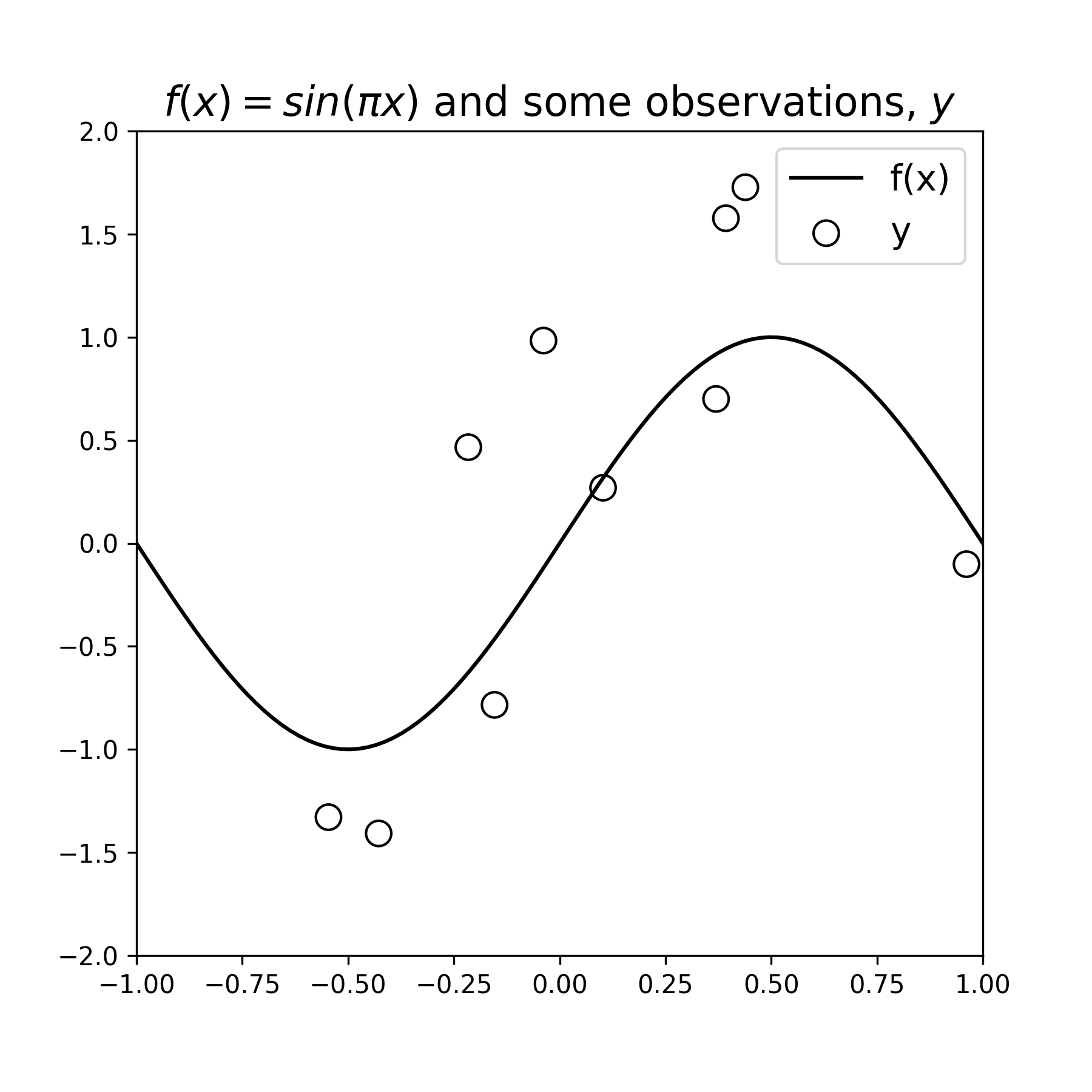
Below we define the function \(f(x)\) and display it, then draw a few observation samples \(y\), and display them as well:
Figure 1: A data-generating function \(f(x)\) and some noisy samples \(y\). The samples exibit a noise variance \(\sigma_{\epsilon}^2=1\)
# Frontmatter
import numpy as np
np.random.seed(123)
MARKER_SIZE = 100
DATA_COLOR = 'black'
ERROR_COLOR = 'darkred'
POLYNOMIAL_FIT_COLORS = ['orange', 'royalblue', 'darkgreen']
LEGEND_FONTSIZE = 14
TITLE_FONTISIZE = 16
N_OBSERVATIONS = 10
NOISE_STD = 1.
x = 2 * (np.random.rand(N_OBSERVATIONS) - .5)
x_grid = np.linspace(-1, 1, 100)
def f(x):
"""Base function"""
return np.sin(x * np.pi)
def sample_fx_data(shape, noise_std=NOISE_STD):
return f(x) + np.random.randn(*shape) * noise_std
def plot_fx_data(y=None):
"""Plot f(x) and noisy samples"""
y = y if y is not None else sample_fx_data(x.shape)
fig, axs = plt.subplots(figsize=(6, 6))
plt.plot(x_grid, f(x_grid), color=DATA_COLOR, label='f(x)')
plt.scatter(x, y, s=MARKER_SIZE, edgecolor=DATA_COLOR, facecolors='none', label='y')
# Plot the data
y = sample_fx_data(x.shape)
plot_fx_data(y)
plt.legend(fontsize=14)
plt.title(f'$f(x) = sin(\pi x)$ and some observations, $y$', fontsize=16)
plt.xlim([-1, 1])
plt.ylim([-2, 2])
Our goal is to characterized the function \(f(x)\), but we don’t know the function form of \(f(x)\), we must instead estimate some other function \(g(x)\) that we believe will provide an accurate approximation to \(f(x)\). The function \(g(x)\) is called an estimator of \(f(x)\). In general, an estimator is some parameterized model that can capture a wide range of functional forms. One such class of estimators is the weighted combination of ordered polynomials:
\[g_D(x) = \theta_0 + \theta_1x + \theta_2x^2 + \dots \theta_D x^D\]As the polynomial order \(D\) increases, the functions \(g_D(x)\) are able to capture increasingly complex behavior. For example, \(g_0(x)\) desribes a horizontal line with an adjustable vertical offset \(\theta_0\), \(g_1(x)\) desribes a line with adjustable vertical offset and adjustable linear slope \(\theta_1\), \(g_2(x)\) describes a function that also includes a weight on the quadratic term \(\theta_2\). We thus try to fit the values of the parameters for a given estimator \(g_D(x)\) to best account for observed data in the hopes that we will also accurately approximate \(f(x)\).
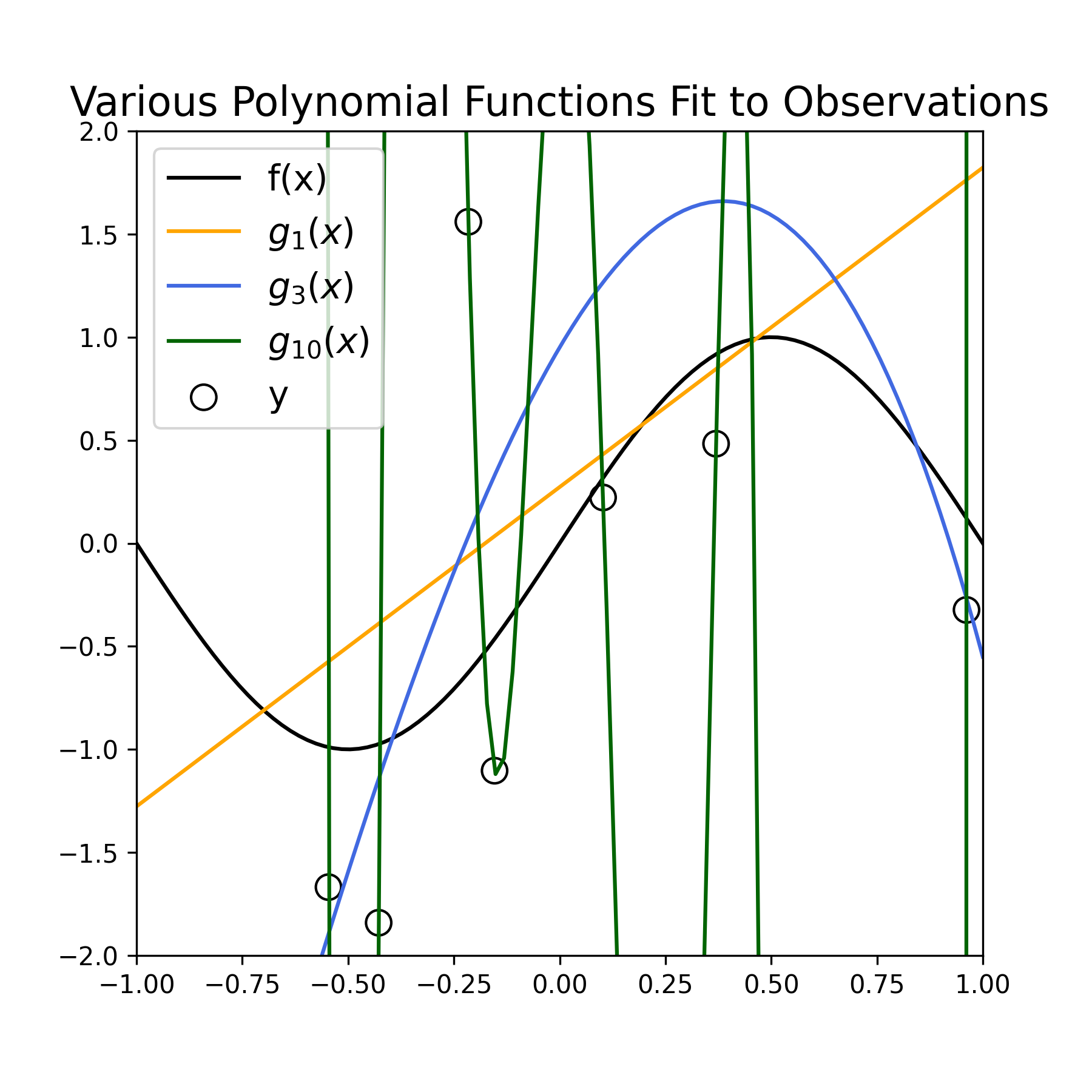
Below we estimate the parameters of three polynomial model functions of increasing complexity (using Numpy’s polyfit
) to the sampled data displayed above. Specifically, we estimate the functions \(g_1(x)\), \(g_3(x)\), and \(g_{10}(x)\).
Figure 2: Fitting various polynomial estimators \(g_D(x)\) fit to noisy samples \(y\), for \(D = (1, 3, 10)\).
plot_fx_data(y)
polynomial_degrees = [1, 3, 10]
theta = {}
fit = {}
for ii, degree in enumerate(polynomial_degrees):
# Note: we should get an overconditioned warning for degree 10 because of extreme overfitting
theta[degree] = np.polyfit(x, y, degree)
fit[degree] = np.polyval(theta[degree], x_grid)
plt.plot(x_grid, fit[degree], POLYNOMIAL_FIT_COLORS[ii], label=f"$g_(x)$")
plt.legend(fontsize=LEGEND_FONTSIZE)
plt.xlim([-1, 1])
plt.ylim([-2, 2])
plt.title("Various Polynomial Functions Fit to Observations", fontsize=TITLE_FONTISIZE)
Qualitatively, we see that the estimator \(g_1(x)\) (orange line) provides a poor fit to the observed data, as well as a poor approximation to the function \(f(x)\) (black curve). We see that the estimator \(g_{10}(x)\) (green curve) provides a very accurate fit to the data points, but varies wildly to do so, and therefore provides an inaccurate approximation of \(f(x)\). Finally, we see that the estimator \(g_3(x)\) (blue curve) provides a fairly good fit to the observed data, and a much better job at approximating \(f(x)\).
Our original goal was to approximate \(f(x)\), not the data points per se. Therefore \(g_3(x)\), at least qualitatively, provides a more desirable estimate of \(f(x)\) than the other two estimators. The fits for \(g_1(x)\) and \(g_{10}(x)\) are examples of “underfitting” and “overfitting” to the observed data, respectively:
The model fits for \(g_D(x)\) discussed above were based on a single, randomly-sampled data set of observations \(y\). However, because \(\epsilon\) is a random variable, there are in principle a potentially infinite number of ranndom data sets that can be observed. In order to determine a good model of \(f(x)\), it would be helpful to have an idea of how an estimator will perform on any or all of these potential datasets. To get an idea of how each of the estimators discussed above performs in general we can repeat the model fitting procedure for many data sets.
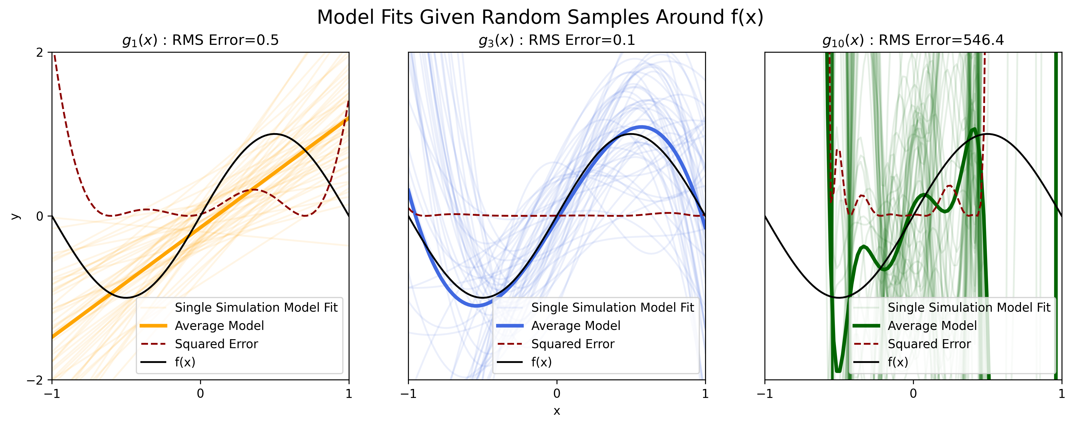
Here we perform such an analyses, sampling 50 independent data sets according to Equation 1, then fitting the parameters for the polynomial functions of model order \(D = (1,3,10)\) to each dataset.
Figure 3: Fitting various polynomial estimators \(g_D(x)\) fit to noisy samples \(y\), for \(D = (1, 3, 10)\).
from collections import defaultdict
n_simulations = 50
simulation_fits = defaultdict(list)
for sim in range(n_simulations):
# Start from same samples
y_simulation = sample_fx_data(x.shape)
for degree in polynomial_degrees:
# Note: we should get an overconditioned warning
# for degree 10 because of extreme overfitting
theta_tmp = np.polyfit(x, y_simulation, degree)
simulation_fits[degree].append(np.polyval(theta_tmp, x_grid))
def error_function(pred, actual):
return (pred - actual) ** 2
fig, axs = plt.subplots(1, 3, figsize=(15, 5))
for ii, degree in enumerate(polynomial_degrees):
plt.sca(axs[ii])
for jj, fit in enumerate(simulation_fits[degree]):
label = 'Single Simulation Model Fit' if jj == 0 else None
plt.plot(x_grid, fit, color=POLYNOMIAL_FIT_COLORS[ii], alpha=.1, label=label)
average_fit = np.array(simulation_fits[degree]).mean(0)
squared_error = error_function(average_fit, f(x_grid))
rms = np.sqrt(mean(squared_error))
plt.plot(x_grid, average_fit, color=POLYNOMIAL_FIT_COLORS[ii], linewidth=3, label='Average Model')
plt.plot(x_grid, squared_error, '--', color=ERROR_COLOR, label='Squared Error')
plt.plot(x_grid, f(x_grid), color='black', label='f(x)')
plt.yticks([])
if ii == 1:
plt.xlabel('x')
elif ii == 0:
plt.ylabel('y')
plt.yticks([-2, 0, 2])
plt.xlim([-1, 1])
plt.ylim([-2, 2])
plt.xticks([-1, 0, 1])
plt.title(f"$g_(x)$ : RMS Error={np.round(rms, 1)}")
plt.legend(loc='lower right')
plt.suptitle('Model Fits Given Random Samples Around f(x)', fontsize=TITLE_FONTISIZE)
The lightly-colored curves in each of the three plots above are an individual polynomial model fit to one of the 50 sampled data sets. The darkly-colored curve in each plot is the average over the 50 individual fits. The dark curve is the true, underlying function \(f(x)\).
We see that for the estimator \(g_1(x)\) (light orange curves), model fits do not vary too dramatically from data set to data set. Thus the averaged estimator fit over all the data sets (dark orange curve), formally written as \(\mathbb E[g(x)]\), is similar (in terms of slope and vertical offset) to each of the individual fits.
A commonly-used statistical metric that tries to assess the average accuracy of an estimator \(g(x)\) at approximating a target function \(f(x)\) is what is called the bias of the estimator. Formally defined as:
\[\text{bias} = \mathbb E[g(x)] - f(x)\]The bias describes how much the average estimator fit over many datasets \(\mathbb E[g(x)]\) deviates from the value of the actual underlying target function \(f(x)\).
We can see from the plot for \(g(x)_1\) that \(\mathbb E[g_1(x)]\) deviates significantly from \(f(x)\). Thus we can say that the estimator \(g_1(x)\) exhibits large bias when approximating the function \(f(x)\).
When averaging over the individual fits for the estimator \(g_3(x)\) (blue curves), we find that the average estimator \(\mathbb E[g_3(x)]\) (dark blue curve) accurately approximates the true function \(f(x)\), indicating that the estimator \(g_3(x)\) has low bias.
Another common statistical metric attempts to capture the average consistency of an estimator when fit to multiple datasets. This metric, referred to as the variance of the estimator is formally defined as
\[\text{variance} = \mathbb E[(g(x)-\mathbb E[g(x)])^2]\]The variance is the expected (i.e. average) squared difference between any single dataset-dependent estimate of \(g(x)\) and the average value of \(g(x)\) estimated over all datasets, \(\mathbb E[g(x)]\).
According to the definition of variance, we can say that the estimator \(g_1(x)\) exhibits low variance because the each individual \(g_1(x)\) is fairly similar across datasets.
Investigating the results for the estimator \(g_{10}(x)\) (green curves), we see that each individual model fit varies dramatically from one data set to another. Thus we can say that this estimator exhibits high variance.
We established earlier that the estimator \(g_3(x)\) provided a qualitatively better fit to the function \(f(x)\) than the other two polynomial estimators for a single dataset. It appears that this is also the case over many datasets. We also find that estimator \(g_3(x)\) exhibits low bias and low variance, whereas the other two, less-desirable estimators, have either high bias or high variance. Thus it would appear that having both low bias and low variance is a reasonable criterion for selecting an accurate model of \(f(x)\).
Included in each of the three plots in Figure 3 is a dashed red line representing the squared difference between the average estimator \(\mathbb E[g_D(x)]\) and the true function \(f(x)\). Calculating squared model errors is a common practice for quantifying the goodness of a model fit. If we were to calculate the expected value of each of the dashed red lines–assuming that all \(N\) values in an array of independent variables \(\mathbf x\) are equally likely to occur–we would obtain a single value for each estimator that is the mean squared error (MSE) between the expected estimator and the true function:
\[\mathbb E[(\mathbb E[g(\mathbf{x})]-f(\mathbf{x}))^2] = \frac{1}{N}\sum_{i=1}^N (\mathbb E[g(x_i)]-f(x_i))^2\]For the estimator \(g_3(x)\), the MSE will be very small, as the dashed black curve for this estimator is near zero for all values of \(\mathbf x\). The estimators \(g_1(x)\) and \(g_{10}(x)\) would have substantially larger MSE values. Now, because exhibiting both a low MSE, as well as having both low bias and variance are indicative of a good estimator, it would be reasonable to assume that squared model error is directly related to bias and variance. The next section provides some formal evidence for this notion.
For a given estimator \(g(x)\) fit to a data set of \(x\text{-}y\) pairs, we would like to know, given all the possible datasets out there, what is the expected prediction error we will observe for a new data point \(x^*\), \(y^*\) = \(f(x^*) + \epsilon\). If we define prediction error to be the squared difference in model prediction \(g(x^*)\) and observations \(y^*\), the expected prediction error is then:
\[\mathbb E[(g(x^*) - y^*)^2]\]If we expand this a little and use a few identities, something interesting happens:
\[\begin{align} \mathbb E[(g(x^*) - y^*)^2] &= \mathbb E[g(x^*)^2-2g(x^*)y^*+y^{*2}] \tag{2} \\ & = \mathbb E[g(x^*)^2] - 2\mathbb E[g(x^*)y^*] + \mathbb E[y^{*2}] \tag{3} \\ & = \mathbb E[(g(x^*) - \mathbb E[g(x^*)])^2] + \mathbb E[g(x^*)]^2 \\ & \;\;\;\;-2 \mathbb E[g(x^*)]f(x^*) \\ & \;\;\;\;+ \mathbb E[(y^*-f(x^*))^2] + f(x^*)^2 \tag{4} \end{align}\]where we have applied the following Lemma to the first and third terms of Equation 3, and use the fact to \(\mathbb E[y] = f(x)\) (Think of averaging over an infinite number of datasets sampled from y; all noise will average out, leaving \(f(x)\)). Rearranging Equation 4, we obtain:
\[\mathbb E[(g(x^*) - \mathbb E[g(x^*)])^2] + (\mathbb E[g(x^*)]^2 - 2 \mathbb E[g(x^*)]f(x^*) + f(x^*)^2) + \mathbb E[(y^*-f(x^*))^2] \tag{5}\]which can be further simplified by reversing a polynomial expansion and highlighting three terms
\[\color{green}{\mathbb E[(g(x^*) - \mathbb E[g(x^*)])^2]} + \color{blue}{( \mathbb E[g(x^*)]-f(x^*))^2} + \color{red}{\mathbb E[(y^*-f(x^*))^2]} \tag{6}\]Here we find that the expected prediction error on new data \((x^*,y^*)\) (in the squared differences sense) is the combination of these three terms: the estimator variance, squared-bias, and the observation noise variance. This take-home is important in that it states that the expected prediction error on new data can be used as a quantitative criterion for selecting the best model from a candidate set of estimators!
It turns out that, given \(N\) new data points \((\mathbf x^*,\mathbf y^*)\), the expected prediction error can be easily approximated as the mean squared error over data pairs:
\[\mathbb E[(g(\mathbf x^*) - \mathbf y^*)^2] \approx \frac{1}{N}\sum_{i=1}^N(g(x_i^*)-y_i^*)^2\]thus giving us a convenient metric for determining the best model out of a set of candidate estimators.
Below we demonstrate the findings presented above with another set of simulations. We simulate 100 independent datasets, each with 25 \(x\text{-}y\) pairs; the samples \(y\) have a noise variacne \(\sigma_{\epsilon}^2=\sigma_{\text{noise}}^2=0.25\). We then partition each dataset into two non-overlapping sets:
We then fit the parameters for estimators of varying complexity. Complexity is varied by using polynomial functions that range in model order from 1 (least complex) to 12 (most complex). We then calculate and display the squared bias, variance, and prediction error on testing set for each of the estimators:
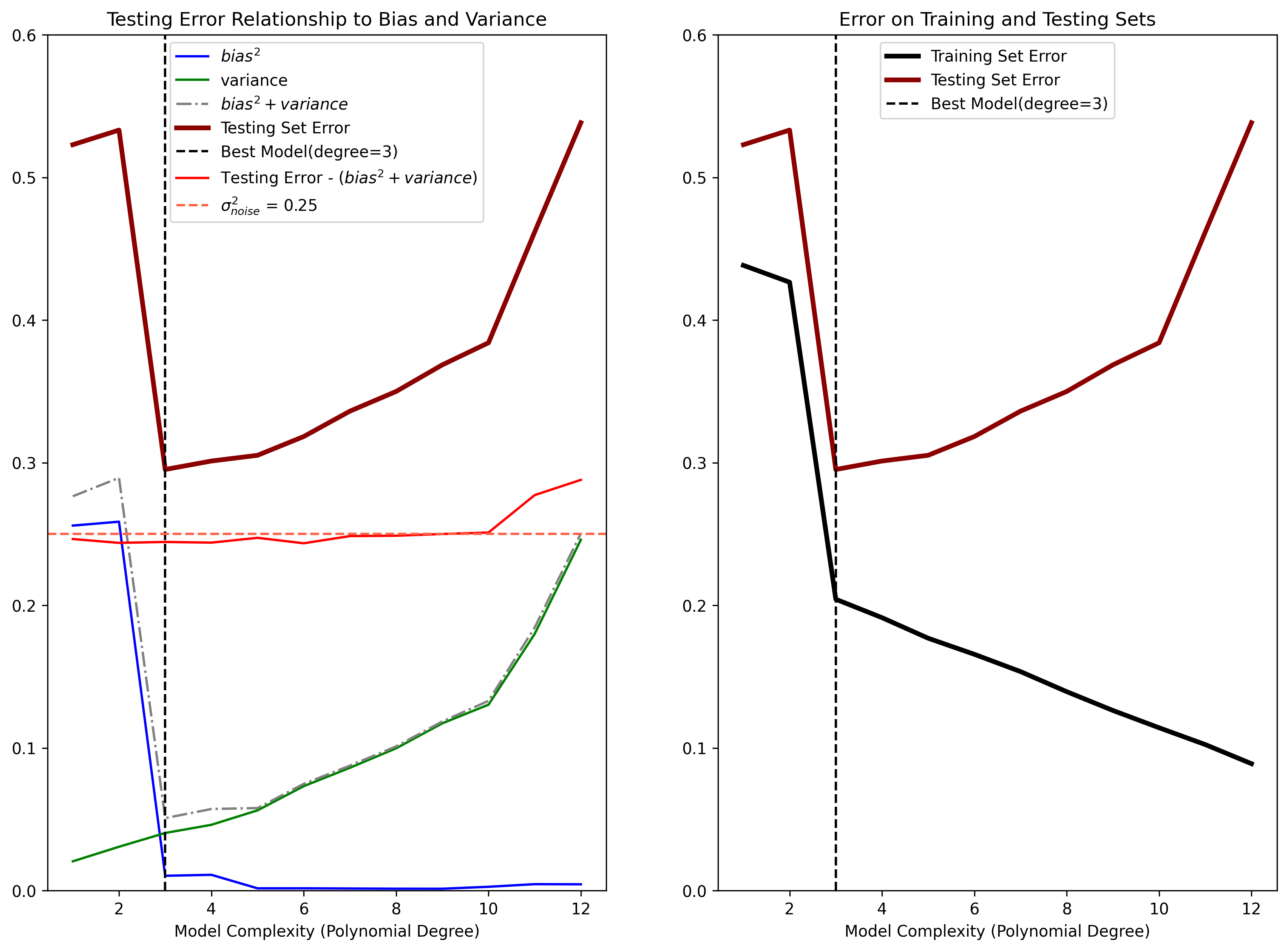
Figure 4: (Left) Demonstration of how estimator bias and variance contribute to the mean squared error on the Testing Set. The Testing Set error (dark red) can be broken down into a three components: the squared bias (blue) of the estimator, the estimator variance (green), and the noise variance \(\sigma_{noise}^2\) (red). The “best” model (polynomial degree \(D=3\)) has the optimal balance of low bias and low variance. Note that the noise variance is considered a lower bound on the Testing Set error, as it cannot be accounted for by any model. (Right) Demonstration of overfitting when the model complexity suprasses the optimal bias-variance tradeoff. Models with a complexity above \(D=3\) are able to fit the Training Set data better, but at the expense of not generalizing to the Testing Set, resulting in increasing generalization error.
np.random.seed(124)
n_observations_per_dataset = 25
n_datasets = 100
max_poly_degree = 12 # Maximum model complexity
model_poly_degrees = range(1, max_poly_degree + 1)
NOISE_STD = .5
percent_train = .8
n_train = int(np.ceil(n_observations_per_dataset * percent_train))
# Create training/testing inputs
x = np.linspace(-1, 1, n_observations_per_dataset)
x = np.random.permutation(x)
x_train = x[:n_train]
x_test = x[n_train:]
# logging variables
theta_hat = defaultdict(list)
pred_train = defaultdict(list)
pred_test = defaultdict(list)
train_errors = defaultdict(list)
test_errors = defaultdict(list)
# Loop over datasets
for dataset in range(n_datasets):
# Simulate training/testing targets
y_train = f(x_train) + NOISE_STD * np.random.randn(*x_train.shape)
y_test = f(x_test) + NOISE_STD * np.random.randn(*x_test.shape)
# Loop over model complexities
for degree in model_poly_degrees:
# Train model
tmp_theta_hat = polyfit(x_train, y_train, degree)
# Make predictions on train set
tmp_pred_train = polyval(tmp_theta_hat, x_train)
pred_train[degree].append(tmp_pred_train)
# Test predictions
tmp_pred_test = polyval(tmp_theta_hat, x_test)
pred_test[degree].append(tmp_pred_test)
# Mean Squared Error for train and test sets
train_errors[degree].append(np.mean(error_function(tmp_pred_train, y_train)))
test_errors[degree].append(np.mean(error_function(tmp_pred_test, y_test)))
def calculate_estimator_bias_squared(pred_test):
pred_test = np.array(pred_test)
average_model_prediction = pred_test.mean(0) # E[g(x)]
# (E[g(x)] - f(x))^2, averaged across all trials
return np.mean((average_model_prediction - f(x_test)) ** 2)
def calculate_estimator_variance(pred_test):
pred_test = np.array(pred_test)
average_model_prediction = pred_test.mean(0) # E[g(x)]
# (g(x) - E[g(x)])^2, averaged across all trials
return np.mean((pred_test - average_model_prediction) ** 2)
complexity_train_error = []
complexity_test_error = []
bias_squared = []
variance = []
for degree in model_poly_degrees:
complexity_train_error.append(np.mean(train_errors[degree]))
complexity_test_error.append(np.mean(test_errors[degree]))
bias_squared.append(calculate_estimator_bias_squared(pred_test[degree]))
variance.append(calculate_estimator_variance(pred_test[degree]))
best_model_degree = model_poly_degrees[np.argmin(complexity_test_error)]
# Visualizations
fig, axs = plt.subplots(1, 2, figsize=(14, 10))
## Plot Bias^2 + variance
plt.sca(axs[0])
plt.plot(model_poly_degrees, bias_squared, color='blue', label='$bias^2$')
plt.plot(model_poly_degrees, variance, color='green', label='variance')
plt.plot(model_poly_degrees, np.array(bias_squared) + np.array(variance), linestyle='-.', color='gray', label='$bias^2 + variance$')
plt.plot(model_poly_degrees, complexity_test_error, label='Testing Set Error', linewidth=3, color=ERROR_COLOR)
plt.axvline(best_model_degree, linestyle='--', color='black', label=f'Best Model(degree={best_model_degree})')
plt.plot(model_poly_degrees, np.array(complexity_test_error) - (np.array(bias_squared) + np.array(variance)), color='red', label='Testing Error - ($bias^2 + variance$)')
plt.axhline(NOISE_STD **2, color='tomato', linestyle='--', label=f'$\sigma_^2$ = {round(NOISE_STD**2, 3)}')
plt.xlabel('Model Complexity (Polynomial Degree)')
plt.ylim([0, .6]);
plt.legend()
plt.title('Testing Error Relationship to Bias and Variance')
## Plot Train / Test Set Error
plt.sca(axs[1])
plt.plot(model_poly_degrees, complexity_train_error, label='Training Set Error', linewidth=3, color=DATA_COLOR)
plt.plot(model_poly_degrees, complexity_test_error, label='Testing Set Error', linewidth=3, color=ERROR_COLOR)
plt.axvline(best_model_degree, linestyle='--', color='black', label=f'Best Model(degree={best_model_degree})')
plt.ylim([0, .6]);
plt.xlabel('Model Complexity (Polynomial Degree)')
plt.title('Error on Training and Testing Sets')
plt.legend(loc='upper center')
In the left subpanel of Figure 4 we see how, as the model complexity increases, the estimator variance (green curve) also increases. Additionally, as model complexity increases, the squared bias (blue curve) decreases. Thus there is a tradeoff between bias and variance that comes with model complexity:
In this example, we highlight the best estimator in terms of prediction error on the testing set (dark red curve) with a dashed black vertical line. The best estimator corresponds to a polynomial model of order of \(D=3\). Notice that the vertical black line is located where function defined by the sum of the squared bias and variance (dashed gray curve) is also at a minimum.
It’s also important to notice that the sum of the squared bias and variance has the same shape as the curve defined by the mean squared prediction error on the testing set. This exemplifies how the error on novel data can be used as a proxy for determining the best estimator from a candidate set based on squared bias and variance. The noise term in Equation 6 is also represented in the left subpanel of Figure 4 as the red curve. This curve was calculated by taking the difference between the Testing Set error and the sum of the variance and squared bias. We can see that the noise term is roughly constant, and equivalent to underlyng the variance of the observations \(\sigma_{\text{noise}}^2\) (indicated by the dashed red line).
It’s important to be clear that all of the simulated results above are based on evaluating prediction error on novel data, not used to estimate model parameters. It turns out that assessing a model performance based on prediction error calculated on the same data used to estimate the model parameters is highly problematic, as it causes models to always “overfit.” In plain terms, overfitting means that we will always favor a more complex estimator if we assess goodness of model fits on the training data, as a more complex model will be better able to capture small, random trends in the data due to noise.
This overfitting phenomenon is demonstrated in the right side of Figure 4. For the same simulation data as in the left of Figure 4, we plot the error calculated on the Training set (black curve) along with the error calculated on the testing set (red curve). We also identify the best estimator based on the Testing Set Error.
We see here that as model complexity increases, the error calculated on the training set continues to decrease, whereas the error on the testing set increases past the optimal polynomial order \(D=3\). We showed above that error calculated on the testing set is the true indicator of how well an estimator will generalize to new data points. The error calculated on the training set strongly disagrees with the error calculated on the testing set after the optimal model complexity has been reached. Since, in general, the whole point of modeling a data set is to generalize to novel data, assessing model predictions on the training set data should be avoided.
In this post we discussed how the bias and variance of an estimator are related to squared prediction error on the testing set. Though we focused on regression, these concepts can also be applied to classification problems. We found that an optimal estimator will have both low variance and low bias. We further found that information about squared bias and variance is contained in expected prediction error calculated on a testing set of data not used to fit a model’s parameters.
The concepts of estimator bias and variance are generally only clear in the context of an ensemble of datasets. However, in real-world applications, there is generally only a single observed dataset. In such cases the roles of bias and variance are less obvious (though, it is possible to calculate estimates of variance and bias using resampling methods such as bootstrapping).
However, the direct connection we made between bias, variance with the mean-squared error calculated on a testing set give us a direct means for assessing a group of candidate estimators in light of a single data set. We only need to partition the available data set into a Training Set used to fit model parameters and a Testing Set used to assess prediction accuracy.
Comparing prediction accuracy across potential estimators is equivalent to assessing biases and variances of the estimators across many datasets. Note that resampling methods such as cross-validation can prove helpful here, particularly when the amount of observed data is small.
This post is a refactor of content with the same title originally posted on The Clever Machine Wordpress blog.
]]>If we expand the first expression on the right-hand side of Equation 1:
\[\begin{align} \mathbb E [(X - \mathbb E[X])^2] &= \mathbb E[X^2-2X\mathbb E[X]+\mathbb E [X]^2] \\ &= \mathbb E[X^2] - 2\mathbb E[X] \mathbb E [\mathbb E [X]] + \mathbb E [\mathbb E [X]^2]. \tag{2} \end{align}\]If we note that \(\mathbb E[X]\) is a constant, then \(\mathbb E[\mathbb E[X]]\) is also a constant, namely \(\mathbb E[X]\). Taking this into account Equation 2 simplifies to:
\[\begin{align} \mathbb E[(X - \mathbb E[X])^2] &= \mathbb E[X^2] - 2\mathbb E[X] \mathbb E[X] + \mathbb E[X]^2 \\ &= \mathbb E[X^2] - 2\mathbb E[X]^2 + \mathbb E[X]^2 \\ &= \mathbb E[X^2] - \mathbb E[X]^2 \tag{3} \end{align}\]Plugging Equation 3 back into the right-hand side of Equation 1 gives
\[\begin{align} \mathbb E[(X - \mathbb E[X])^2] + \mathbb E[X]^2 &= \mathbb E[X^2] - \mathbb E[X]^2 + \mathbb E[X]^2 \\ &= \mathbb E[X^2] , \tag{4} \end{align}\]thus giving the desired result.
]]>