Who Needs Backpropagation? Computing Word Embeddings with Linear Algebra
Word embeddings provide numerical representations of words that carry useful semantic information about natural language. This has made word embeddings an integral part of modern Natural Language Processing (NLP) pipelines and language understanding models. Common methods used to compute word embeddings, like word2vec, employ predictive, neural network frameworks. However, as we’ll show in this post, we can also compute word embeddings using a some basic frequency statistics, a little information theory, and our good old friend from linear algebra, Singular Value Decomposition.
Motivation
Building computational systems that can interact naturally with humans requires computers to be able to process natural language, i.e. words. Words carry information about real-world, semantic entities, actions, or notions. However, computers do not operate in the space of semantics, but instead employ numerical operations. Therefore in order to build useful computer-human-language interfaces, we need a way of numerically representing words and their semantics.
The classic way of representing a word numerically is to use a “1-of-\(K\)” or “one-hot” encoding (Figure 1, Top Left). This encoding uses a sparse vector of length-\(K\), representing each of the words in a length-\(K\) vocabulary. The vector is filled with zeros except a single value of one located at the index associated with the represented word. One can think of the 1-of-\(K\) encoding acting like a vectorized indicator variable for the presence of a word.
This 1-of-\(K\) encoding is simple and provides an orthogonal set of features to represent words. Consequently it has been the backbone of many NLP models for decades. However, 1-of-\(K\) encoding can be inefficient in that the cardinality of the feature space can become quite large for large vocabularies, quickly running into the curse of dimensionality that makes so many machine learning problems ill-posed, or require tons of observations to obtain good parameter estimates. Additionally, the 1-of-\(K\) encoding carries little semantic information about the vocabulary it represents.
Enter Word Embeddings
In recent years, a more compact alternative to 1-of-\(K\) encoding, which carries more semantic information, has been to use word embeddings. Rather than large, sparse vectors, word embeddings provide for each word a dense vector with length that is generally orders of magnitude smaller than the 1-of-\(K\) encoding (generally on the order of a few hundred dimensions or less).
There are a number of ways to derive dense word embeddings, but by far most common approach is to use the word2vec algorithm. This post won’t go into the details of word2vec, but basic ideas goes like this: The word2vec algorithm trains a neural network that is optimized on a corpus of sentences. Given a query word \(w\) sampled from one of the corpus sentences, the network’s task is to predict each of the words \(c\) that are located within a context window \(C\) surrounding the query word (Figure 1, Right).
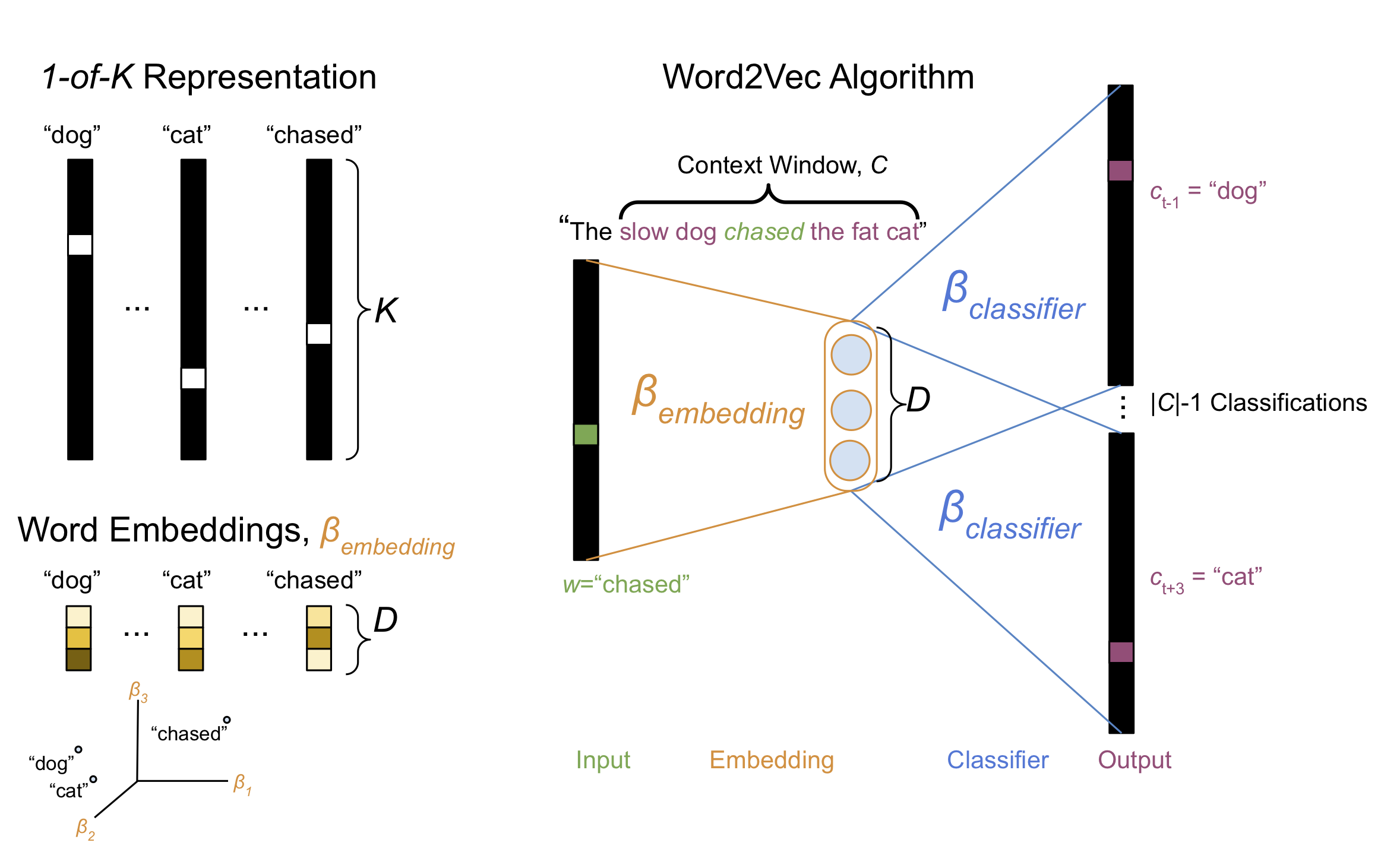
Figure 1, Various methods for representing words numerically. Top Left, “1-of-\(K\)” encoding represents each word as a sparse vector of \(K\) entries with only a single one-valued entry indicating the presence of a particular word. Right, The word2vec algorithm trains a two-layer neural network to predict, given a sentence and a query word from that sentence \(w\), the words \(c\) located within a context window \(C\) surrounding \(w\). Bottom Left, Once the neural network has been optimized, each row of the \(K \times D\) weight matrix in the first hidden layer of the neural network \(\beta_{embedding}\) provides a dense vector representation for each of the \(K\) words in the vocabulary.
The input to the neural network is the 1-of-\(K\) representation of the query word and each of the target context words are represented as, you guessed it 1-of-\(K\) encodings. For each query word there are \(\mid C \mid - 1\) classification targets, one for each context word \(c\). The neural network uses a hidden layer comprised of \(D\) units, and thus there is a matrix of parameters \(\beta_{embedding} \in \mathbb{R}^{K \times D}\) that linearly maps each word into a latent space of size \(D \ll K\). After the network has converged, each row of the first layer of weights \(\beta_{embedding}\) provides for each word a dense embedding vector representation of size \(D\), rather than \(K\) (Figure 1, Bottom Left).
It turns out that the resulting word embedding vectors capture rich semantic information about the words in the corpus. In particular, words that are semantically similar occupy nearby locations in the \(D\)-dimensional space (Figure 1, Bottom Left). Additionally, semantic relationships amongst words are encoded by displacements in the embedding space.
Calculating Information-theoretic Word Embeddings with SVD
Calculating word embeddings using the word2vec algorithm requires building and training a neural network, which in turn involves a considerable amount of calculus necessary for gradient-based parameter optimization. It turns out that there is a simpler way to calculate equivalent word vectors using a little information theory and linear algebra.1 Before digging into this method, let’s first introduce a few basic concepts.
Marginal and Joint Probabilities
The foundation of information theory is probability, and specifically relevant for this post, marginal and joint probabilities. The marginal probability of a word \(p(w_i)\) within a corpus of text is simply the number of times the word occurs \(N(w_i)\) divided by the total number of word occurrences in the corpus \(\sum_k N(w_k)\):
\[p(w_i) = \frac{N(w_i)}{\sum_k N(w_k)} \tag{1}\]In this post we refer to \(N(w_i)\) as unigram frequency, as it is a count of the number of times a single word, or “unigram”, occurs in the corpus.
Unigram Frequency Python Code
from collections import Counter
class UnigramFrequencies(object):
    """Simple Unigram frequency calculator.
    Parameters
    ----------
    documents : list[list[str]]
        A list of documents, each document being a list of strings
    """
    def __init__(self, documents=None):
        self.unigram_counts = Counter()

        for ii, doc in enumerate(documents):
            self.unigram_counts.update(doc)

        self.token_to_idx = {tok: indx for indx, tok in enumerate(self.unigram_counts.keys())}
        self.idx_to_token = {indx: tok for tok, indx in self.token_to_idx.items()}

    def __getitem__(self, item):
        if isinstance(item, str):
            return self.unigram_counts[item]
        elif isinstance(item, int):
            return self.unigram_counts[self.idx_to_token[item]]
        raise ValueError(f"type {type(item)} not supported")
The joint probability of word \(w_i\) and another word \(w_j, j\neq i\) is simply the number of times the words co-occur \(N(w_i, w_j)\) divided by the total number of words:
\[p(w_i, w_j) = \frac{N(w_i, w_j)}{\sum_k N(w_k)} \tag{2}\]There are many possible definitions of co-occurrence, but in this post we’ll use skipgram frequencies to define co-occurrence. Skipgrams define the joint frequency function \(N(w_i, w_j) = N(w_i, c_{t \pm l})\) as the number of times the context word \(c_{q \pm l}\) occurs within a context window \(C\) that surrounds the target/query word \(w_i\); \(t\) being the token index of the query word and \(l\) being the number of steps preceding or following the query word within the context window (Figure 2, Top Left). This is reminiscent of the context words being individual classification targets in the word2vec approach (Figure 1, Right), but in this case we simply tally up counts of the context words, rather than try to build a classifier to predict the occurrence of the context words.
Skipgram Frequency Python Code
class SkipgramFrequencies(object):
    """Simple skipgrams frequency calculator

    Parameters
    ----------
    documents : list[list[str]]
        A list of documents, each document being a list of strings
    backward_window_size : int
        The number of words to the left used to define the context window
    forward_window_size : int
        The number of words to the right used to define the context window
    """
    def __init__(
        self,
        documents,
        backward_window_size=2,
        forward_window_size=2
    ):
        self.backward_window_size = backward_window_size
        self.forward_window_size = forward_window_size
        self.skipgram_counts = Counter()

        # Independent word frequencies
        self.unigrams = UnigramFrequencies(documents)

        # Conditional word-context frequencies
        for doc_idx, doc in enumerate(documents):
            token_idxs = [self.token_to_idx[token] for token in doc]
            n_document_tokens = len(token_idxs)

            for token_idx, _ in enumerate(token_idxs):
                context_window_start = max(0, token_idx - self.backward_window_size)
                context_window_end = min(n_document_tokens - 1, token_idx + self.forward_window_size) + 1
                context_idxs = [
                    context_idx for context_idx in range(context_window_start,context_window_end)
                    if context_idx != token_idx
                ]
                for context_idx in context_idxs:
                    skipgram = (token_idxs[token_idx], token_idxs[context_idx])
                    self.skipgram_counts[skipgram] += 1

    @property
    def idx_to_token(self):
        return self.unigrams.idx_to_token

    @property
    def token_to_idx(self):
        return self.unigrams.token_to_idx
Pointwise Mutual information
Given the marginal and joint probabilities \(p(w_i)\) and \(p(w_i, w_j)\), we can calculate some powerful information-theoretic quantities. Of particular interest is the Pointwise Mutual Information (PMI):
\[PMI(w_i, w_j) = \log \frac{p(w_i, w_j)}{p(w_i) p(w_j)} \tag{3}\]The PMI matrix offers an intuitive and straight-forward means for calculating associations between words in a corpus: each row gives the amount of information shared between a word and all other words in the corpus. Intuitively, the PMI matrix represents the amount of association between two words. If the two words are independent–i.e. not associated–then the PMI is zero.
Computationally, the PMI is just the log of the joint probability for two words, after being rescaled by the marginal probabilities for each word. Normalizing the joint probability of the two words by the product of their marginal probabilities generates more nuanced representation of their co-occurrence when compared to the raw co-occurrence frequencies. This can be seen in Figure 2, Top Row–the PMI has more small-scale structure thatn the basic skipgram frequency matrix.
PMI Python Code
import numpy as np
from scipy.sparse import csr_matrix

def calculate_pairwise_frequency_matrix(skipgrams, recalculate=False):
    """Given a SkipgramFrequencies instance, returns the associated
    pairwise frequency counts as a sparse matrix
    """
    row_idxs = []
    col_idxs = []
    matrix_values = []
    for (token_idx_1, token_idx_2), skipgram_count in skipgrams.skipgram_counts.items():
        row_idxs.append(token_idx_1)
        col_idxs.append(token_idx_2)
        matrix_values.append(skipgram_count)


def calculate_pmi_matrix(skipgrams, enforce_positive=False, recalculate=False):
    """Given a SkipgramFrequencies instance, returns the associated pointwise
    mutual information (PMI) matrix in sparse (CSR) format
    """
    # Get frequency matrix
    frequency_matrix = calculate_pairwise_frequency_matrix(skipgrams)

    # Precalculate some resusable things
    n_skipgrams = frequency_matrix.sum()
    word_sums = np.array(frequency_matrix.sum(axis=0)).flatten()
    context_sums = np.array(frequency_matrix.sum(axis=1)).flatten()

    # Sparse matrix components
    row_idxs = []
    col_idxs = []
    matrix_values = []

    for (skipgram_word_idx, skipgram_context_idx), skipgram_count in skipgrams.skipgram_counts.items():
        # p(w, c)
        join_probability = skipgram_count / n_skipgrams

        # p(w)
        n_word = context_sums[skipgram_word_idx]
        p_word = n_word / n_skipgrams

        # p(c)
        n_context = word_sums[skipgram_context_idx]
        p_context = n_context / n_skipgrams

        # Pointwise mututal information = log[p(w, c) / p(w)p(c)]
        pmi = np.log(join_probability / (p_word * p_context))

        # Update sparse matrix entries
        row_idxs.append(skipgram_word_idx)
        col_idxs.append(skipgram_context_idx)
        matrix_values.append(pmi)

    return csr_matrix((matrix_values, (row_idxs, col_idxs)))
Information-theoretic Word Embeddings
The PMI matrix is a square, \(K \times K\) matrix. Therefore, if we have a large vocabulary, the PMI matrix can be quite large (though likely sparse). We’ve discussed in a previous post how Singular Value Decomposition (SVD) can be used to compress large matrices. If we apply SVD to the PMI matrix, using a low-rank approximation with \(D \ll K\), we can compute a compact representation of the word association information captured by the PMI matrix. Specifically, we use the left singular vectors \(U\), rescaled by the square root of the singular values \(S\) returned by the SVD (Figure 2, Bottom Row).2
Word Embeddings Python Code
from sklearn.decomposition import TruncatedSVD

def calculate_word_vectors(stats, n_dim=128):
    """Calculates word embedding vectors as the left singular vectors of
    Singular Value Decomposition of the Pointwise Mutual Information Matrix.
    Singular vectors are rescaled by the inverse of the eigenvalues of the
    PMI correlation matrix
    """
    # Get PMI matrix
    if isinstance(stats, SkipgramFrequencies):
        pmi_matrix = calculate_pmi_matrix(stats)
    elif isinstance(stats, csr_matrix):
        pmi_matrix = stats

    # Alternatively, we could use scipy.sparse.linalg.svds / arpack algorithm,
    # but the Halko (2009) algorithm used by default generally scales better
    # on a laptop.
    svd = TruncatedSVD(n_components=n_dim, n_iter=50)

    # Use left singular vectors of PMI, scaled by eigenvalues as embeddings
    U = svd.fit_transform(pmi_matrix)
    return U * np.sqrt(svd.singular_values_)
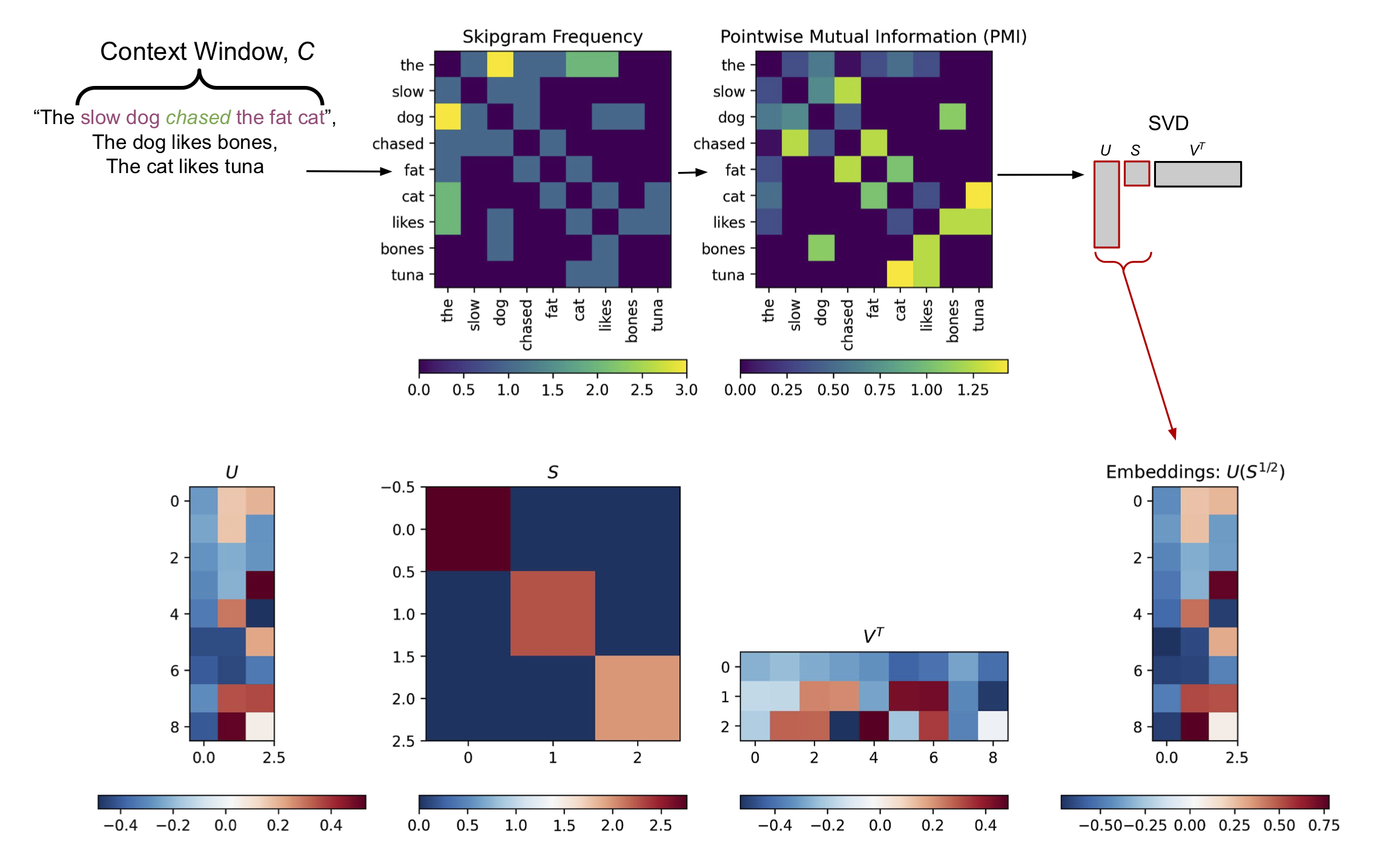
Figure 2, Information-theoretic Word Embeddings from PMI and SVD. Top Row: Unigram frequencies and a \(K \times K\) Skipgram frequency matrix are calculated based a corpus of sentences and a predefined context window \(C\). In this example \(K=9\) is the size of the vocabulary in the corpus. These frequencies are used to calculate a PMI matrix via Equation 3. Bottom Row: Truncated SVD with \(D \ll K\) is applied to the PMI matrix, returning low-rank left singular vectors \(U\) and singular values \(S\). In this toy example \(D=3\). The low-rank left singular vectors are rescaled by the square root of the singular values to return a compressed representation of the PMI matrix of size \(K \times D\). Each row of this low-rank matrix provides an embedding vector for each of the \(K\) words in the vocabulary (Right).
Python Code Used to Generate Figure 2
toy_corpus = [
    'the slow dog chased the fat cat',
    'the dog likes bones',
    'the cat likes tuna'
]
toy_corpus = [c.split(" ") for c in toy_corpus]

# Calcualte the skipgram frequency matrix
toy_skigrams = SkipgramFrequencies(toy_corpus, min_frequency=0)
toy_frequency_matrix = calculate_pairwise_frequency_matrix(toy_skigrams)

# Calculate the PMI matrix
toy_pmi_matrix = calculate_pmi_matrix(toy_skigrams)

# Calculate embeddings
n_embedding_dims = 3  # D

# Calculate associated SVD (redundant, but meh)
U, S_, V = np.linalg.svd(toy_pmi_matrix.todense())

# Truncate at D
S = np.zeros((n_embedding_dims, n_embedding_dims))
np.fill_diagonal(S, S_[:n_embedding_dims])
U = U[:, :n_embedding_dims]
V = V[:n_embedding_dims, :]
toy_embeddings = U @ S ** .5

# Visualizations
fig, axs = plt.subplots(2, 4, figsize=(15, 10))

## Frequency matrix
plt.sca(axs[0][1])
plt.imshow(toy_frequency_matrix.todense())
plt.colorbar(orientation='horizontal', pad=.2)
tics = range(len(toy_skigrams.idx_to_token))
labels = [toy_skigrams.idx_to_token[ii] for ii in tics]
plt.xticks(tics, labels=labels, rotation=90)
plt.yticks(tics, labels=labels)
plt.title("Skipgram Frequency")

## PMI Matrix
plt.sca(axs[0][2])
plt.imshow(toy_pmi_matrix.todense())
plt.colorbar(orientation='horizontal', pad=.2)
plt.xticks(tics, labels=labels, rotation=90)
plt.yticks(tics, labels=labels)
plt.title("Pointwise Mutual Information (PMI)")

## Left singular vectors
plt.sca(axs[1][0])
plt.imshow(U, cmap='RdBu_r')
plt.colorbar(orientation='horizontal')
plt.title('$U$')

## Singular values
plt.sca(axs[1][1])
plt.imshow(S, cmap='RdBu_r')
plt.colorbar(orientation='horizontal')
plt.title("$S$")

## Right singular vectors
plt.sca(axs[1][2])
plt.imshow(V, cmap='RdBu_r')
plt.colorbar(orientation='horizontal')
plt.title("$V^T$")

## Resulting embeddings
plt.sca(axs[1][3])
plt.imshow(toy_embeddings, cmap='RdBu_r')
plt.title("Embeddings: $U(S^{1/2})$")
plt.colorbar(orientation='horizontal')

## Clear unused axes
plt.sca(axs[0][0])
plt.axis('off')
plt.sca(axs[0][3])
plt.axis('off')
This information-theoretic/linear algebra method provides word embeddings that are analogous to those calculated using word2vec.1 Like word2vec embeddings, these information-theoretic embeddings provide a numerical representation that carries semantic information: similar words occupy similar locations in the embedding space, and directionality within the space conveys semantic meaning (Figure 3).
Note that this idea isn’t all that novel. Similar approaches, for example applying SVD directly to the co-occurrence matrix (rather than the PMI matrix), have been used since the 1990s in algorithms like Latent Semantic Indexing to provide word embeddings.3 However, given the current popularity in deep learning and predictive methods, simpler frequency-based and linear algebra-based methods like LSA and the method proposed here have received a lot less attention recently.
Demo: Analyzing the 20Newsgroup Data Set
As a proof of concept, let’s calculate some word embeddings on some real data using the proposed method. For this demo we’ll analyze the 20Newsgroups dataset, which is easily accessible in scikit-learn.
First we load in the data and do some basic preprocessing, including tokenization and stopword and punctuation removal using nltk. This will give a corpus of tokens that we can analyze using the steps outlined above.
Python Code to Load and Preprocess 20Newsgroup Dataset
from sklearn.datasets import fetch_20newsgroups
from string import punctuation
from nltk.corpus import stopwords
from nltk.tokenize import word_tokenize
STOPWORDS = stopwords.words('english')
PUNCTUATION = set(list(punctuation))

def valid_token(token):
    """Basic token filtering for 20 Newgroup task. Results in cleaner embeddings
    and faster convergence. Removes stopwords and any punctuation
    """
    if token in STOPWORDS:
        return False
    if any([t in PUNCTUATION for t in list(token)]):
        return False
    return True

def preprocess(document):
    """Simple preprocessing"""
    return [w for w in word_tokenize(document.lower()) if valid_token(w)]

# For dataset details, see https://scikit-learn.org/0.19/datasets/twenty_newsgroups.html
dataset = fetch_20newsgroups(subset='all', remove=('headers', 'footers'))
corpus = [preprocess(doc) for doc in dataset.data]
From this corpus data we’ll:
- calculate the unigram and skipgram frequencies, followed by
- calculating the associated PMI matrix, followed by
- calculating the associated word embeddings via SVD.
For this example we’ll use an embedding dimensionality of \(D=256\). Notice in the code below that using this dimensionality reduces the PMI matrix from a size of roughly 20k by 20k to a size of 20k by 256, an almost 100x reduction in entries (when in dense format).
Python Code For Calculating 20Newsgroup Word Embeddings
# 1. Calculate unigram / skipgram frequencies of the corpus
skipgram_frequencies = SkipgramFrequencies(corpus)

# 2. Calculate associated PMI matrix
pmi_matrix = calculate_pmi_matrix(skipgram_frequencies)

# 3. Calculate the embedding matrix with D=256
embeddings_matrix = calculate_word_vectors(pmi_matrix, n_dim=256)
print(embeddings_matrix.shape)
# (19699, 256)
In Figure 3 below we visualize the semantic representation of the embedding vectors calculated from the 20Newsgroup corpus by plotting a few query words (red) along with words with the 20 most similar embedding vectors (gray), as measured by cosine similarity. For the visualization we use first two dimensions of the embedding space. We can see that words that are nearby in the embedding space are generally semantically similar.
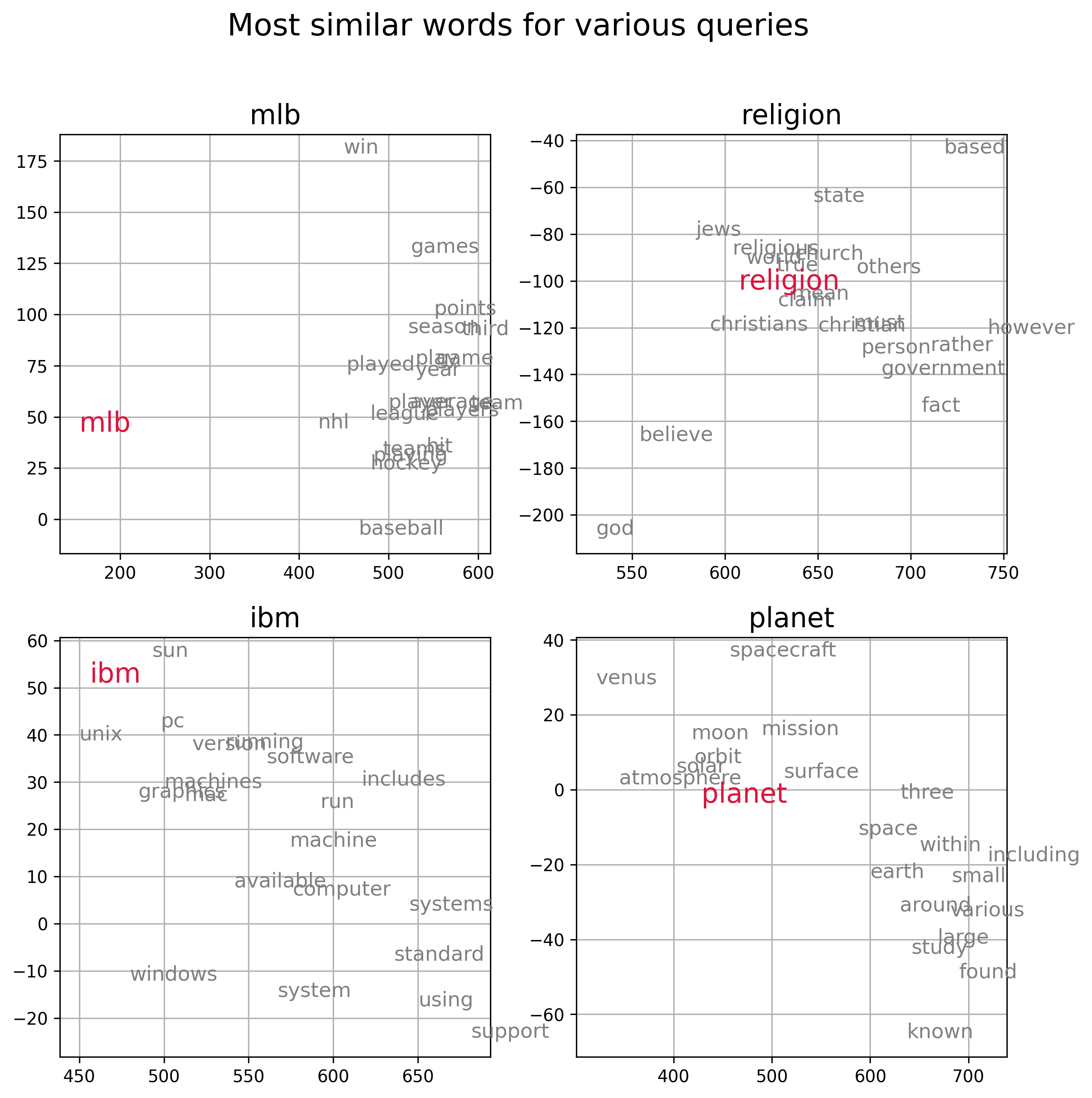
Figure 3, Visualization of information-theoretic embedding vectors derived from the Newsgroup20 data set. Each subpanel plots a query word (red) and the top 20 words with embedding vectors that have the smallest cosine distance from the embedding vector of the query. Word embedding vectors encode semantic relationships amongst words.
Python Code Used to Generate Figure 3
from scipy.spatial.distance import cosine as cosine_similarity
from matplotlib import pyplot as plt

class MatrixNearestNeighborsIndex(object):
    """Simple nearest neighbors index based on a pre-calculated matrix of
    item vectors.

    Parameters
    -----------
    matrix : ndarry or sparse array
        n_items x n_dims matrix of item represation
    idx_to_token : dict
        Mapping between matrix row indices and tokens
    token_to_idx : dict
        Mapping between tokens and matrix row indices

    Notes
    -----
    For simplicity, we could probably infer token_to_idx from idx_to_token,
    but meh
    """
    def __init__(self, matrix, idx_to_token, token_to_idx):
        self.matrix = matrix
        self.idx_to_token = idx_to_token
        self.token_to_idx = token_to_idx

    def most_similar_from_label(self, query_label, n=20, return_self=False):
        query_idx = self.token_to_idx.get(query_label, None)
        if query_idx is not None:
            return self.most_similar_from_index(query_idx, n=n, return_self=return_self)

    def most_similar_from_index(self, query_idx, n=20, return_self=False):
        query_vector = self.get_vector_from_index(query_idx)
        return self.most_similar_from_vector(query_vector, n=n, query_idx=query_idx if not return_self else None)

    def most_similar_from_vector(self, query_vector, n=20, query_idx=None):
        if isinstance(self.matrix, csr_matrix):
            sims = cosine_similarity(self.matrix, query_vector).flatten()
        else:
            sims = self.matrix.dot(query_vector)

        sim_idxs = np.argsort(-sims)[:n + 1]
        sim_idxs = [idx for idx in sim_idxs if (query_idx is None or (query_idx is not None) and (idx != query_idx))]
        sim_word_scores = [(self.idx_to_token[sim_idx], sims[sim_idx]) for sim_idx in sim_idxs[:n]]
        return sim_word_scores

    def get_vector_from_label(self, label):
        query_idx = self.token_to_idx.get(label, None)
        if query_idx is not None:
            return self.get_vector_from_index(query_idx)
        else:
            return np.zeros(self.matrix.shape[1])

    def get_vector_from_index(self, query_idx):
        if isinstance(self.matrix, csr_matrix):
            return self.matrix.getrow(query_idx)
        else:
            return self.matrix[query_idx]

    def __getitem__(self, item):
        if isinstance(item, int):
            return self.get_vector_from_index(item)
        elif isinstance(item, str):
            return self.get_vector_from_label(item)

    def __contains__(self, item):
        return item in self.token_to_idx

# Initialize an nn-index using our embedding vectors
nns = MatrixNearestNeighborsIndex(
    embeddings_matrix,
    skipgram_frequencies.idx_to_token,
    skipgram_frequencies.token_to_idx
)

def plot_label(xy, label, color='gray', fontsize=12):
    plt.plot(xy[0], xy[1], c=color)
    plt.text(xy[0], xy[1], label, c=color, fontsize=fontsize)


labels = ['mlb', 'religion', 'ibm', 'planet']
fig, axs = plt.subplots(2, 2, figsize=(10, 10), dpi=300)

for ii, ax in enumerate(axs.ravel()):
    label = labels[ii]
    plt.sca(ax)
    most_similar = nns.most_similar_from_label(label)
    for sim_label, sim_score in most_similar:
        xy = nns.matrix[nns.token_to_idx[sim_label]][:2]
        plot_label(xy, sim_label)

    xy = nns.matrix[nns.token_to_idx[label]][:2]
    plot_label(xy, label, color='crimson', fontsize=16)
    plt.grid()
    plt.box('on')
    plt.title(label, fontsize=16)

plt.suptitle(f'Most similar words for various queries', fontsize=18)
A common demonstration of how embedding vectors encode semantic information is the “analogy” trick. The idea being that you can apply vector arithmetic to word embeddings to solve analogy tasks such as “King is to Queen as Man is to __”. These analogies would be solved by using vector arithmetic like so:
\[\text{embed}["king"] + \text{embed}["man"] = \text{embed}["queen"] + \text{embed}["woman"] \\ \text{embed}["queen"] = \text{embed}["king"] + \text{embed}["man"] - \text{embed}["woman"]\]I’ve actually never been able to get these analogy tricks to work consistently, and it turns out this isn’t an uncommon experience.4 The size and statistical bias of the corpus used to calculate the embeddings will have a strong influence efficacy these vector arithmetic tricks, which require very similar frequency representations of words to derive similar vectors. Unless you get the exact alignments amongst vectors, you’ll likely not get these tricks to work consistently. This may work for some examples and not for others.
We can still demonstrate the general mechanisms used to calculate these analogies, however. Figure 4 below plots the words involved in the classic royalty analogy introduced above, along with a similar analogy, comparing “boy” to “man” and “girl” to “woman”. In the 20Newsgroup data set we have many more examples of “boy” and “girl” than “queen” in the corpus so we get more consistent results for those examples (it turns out “king” occurs a lot in the data set because it contains many religious, Christian posts that intermix the notion of kings, gods, etc). Specifically, the vectors encoding the displacement from “boy” to “man” and from “girl” to “woman” are nearly parallel and almost equal in length.
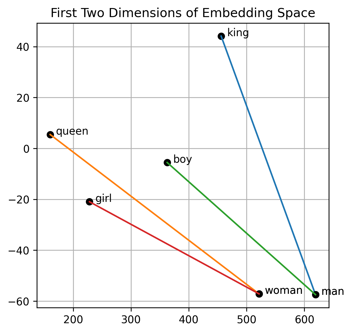
Figure 4, Traversing the embedding space carries semantic information: By definition of SVD the information-theoretic embedding space dimensions are rank-ordered by importance in terms of variance explained amongst the word associations. This allows the embedding space to be easily visualized without the need for dimensionality reduction techniques like PCA. Here we display the two most “important” two dimensions. Similar displacements within the embedding space carry similar semantic information for related words. For example moving from “boy” to “man” (green line) is a very similar vector displacement as moving from “girl” to “woman” (red line). The analogy “king/man” (blue) vs “queen/woman” (orange) analogy referenced in many word embedding papers is also demonstrated.
Python Code Used to Generate Figure 4
def plot_embeddings(sims, pairs):
    fig, axs = plt.subplots(figsize=(5, 5), dpi=300)
    plt.sca(axs)
    for labels in pairs:
        xys = []
        for ii, label in enumerate(labels):
            label_idx = sims.token_to_idx[label]
            x = sims.matrix[label_idx, 0]
            y = sims.matrix[label_idx, 1]

            plt.plot(x, y, 'o', c='black')
            plt.text(x + 10, y, label)
            xys.append([x, y])
        plt.plot([xys[0][0], xys[1][0]], [xys[0][1], xys[1][1]])

    plt.grid()
    plt.title('First 2-dimensions of Embedding Space')

plot_embeddings(nns, [('king', 'man'), ('queen', 'woman'), ('prince', 'boy'), ('princess', 'girl')])
Another way to demonstrate the representation capacity of our word embeddings is to see if we can build an accurate predictive model using these embeddings as machine learning feature vectors. The 20Newsgroups dataset is comprised of approximately 18,000 posts categorized into 20 topics. Below we build a 20-way classifier that predicts the topic of each post based on the average embedding vector calculated across all words in each post.
Python Code For Training the 20Newgroup Classifier
from sklearn.model_selection import train_test_split
from sklearn.linear_model import LogisticRegression
from sklearn.metrics import classification_report

def featurize_document(document, nearest_neighbors):
    vectors = [nearest_neighbors[d] for d in document if d in nearest_neighbors]
    if vectors:
        return np.vstack(vectors).mean(0)
    return np.zeros_like(nearest_neighbors.matrix[0])

def featurize_corpus(corpus, nearest_neighbors):
    vectors = [featurize_document(document, nearest_neighbors) for document in corpus]
    return np.vstack(vectors)

# Featurize the text using our embeddings
features = featurize_corpus(corpus, nns)

# Get train/test sets
X_train, X_test, y_train, y_test, train_idx, test_idx = train_test_split(
    features, dataset.target, range(len(dataset.target))
)

# Fit a Logistic regression classifer
clf = LogisticRegression(max_iter=100, solver='sag').fit(X_train, y_train)

# Get testing set performance
pred_test = clf.predict(X_test)

# Keep copy of actual performance around for plotting effect of training
# set size (Figure 5)
class_report = classification_report(
    y_test, pred_test,
    target_names=dataset.target_names,
    output_dict=True
)

print(classification_report(y_test, pred_test, target_names=dataset.target_names))
The classifier’s performance on all 20 categories is printed below:
                          precision    recall  f1-score   support

             alt.atheism       0.60      0.65      0.62       186
           comp.graphics       0.67      0.65      0.66       248
 comp.os.ms-windows.misc       0.63      0.72      0.67       228
comp.sys.ibm.pc.hardware       0.73      0.64      0.68       241
   comp.sys.mac.hardware       0.74      0.75      0.74       230
          comp.windows.x       0.79      0.72      0.75       262
            misc.forsale       0.70      0.74      0.72       232
               rec.autos       0.85      0.80      0.83       251
         rec.motorcycles       0.83      0.84      0.83       255
      rec.sport.baseball       0.90      0.92      0.91       286
        rec.sport.hockey       0.94      0.94      0.94       258
               sci.crypt       0.82      0.82      0.82       250
         sci.electronics       0.66      0.68      0.67       256
                 sci.med       0.85      0.86      0.85       242
               sci.space       0.86      0.82      0.84       260
  soc.religion.christian       0.70      0.81      0.75       227
      talk.politics.guns       0.66      0.78      0.71       224
   talk.politics.mideast       0.87      0.87      0.87       224
      talk.politics.misc       0.73      0.64      0.68       223
      talk.religion.misc       0.47      0.33      0.39       129

                accuracy                           0.76      4712
               macro avg       0.75      0.75      0.75      4712
            weighted avg       0.76      0.76      0.76      4712
Not too shabby for a super-simple embedding-based classifier! This demonstrates the ability of our 256-dimensional word embedding vectors to capture useful information in text to aid in accurate text classification.
You may notice that we do a lot better on some categories (e.g. rec.sport.hockey) than other categories (e.g. talk.religion.misc). This could be due a few things:
- a few key words capturing a majority of the semantic information in the associated topic
- very consistent posts, with a few, semantically similar words that are highly predictive of the topic
- simply the number of observations available in the training set for each topic
I was curious about the third point, so decided in Figure 5 to plot the testing set F1-score against the number of training set observations used to fit the classifier. It turns out, unsurprisingly, that there is a strong correlation with the amount of training data for a category and the performance of the classifier for that category.
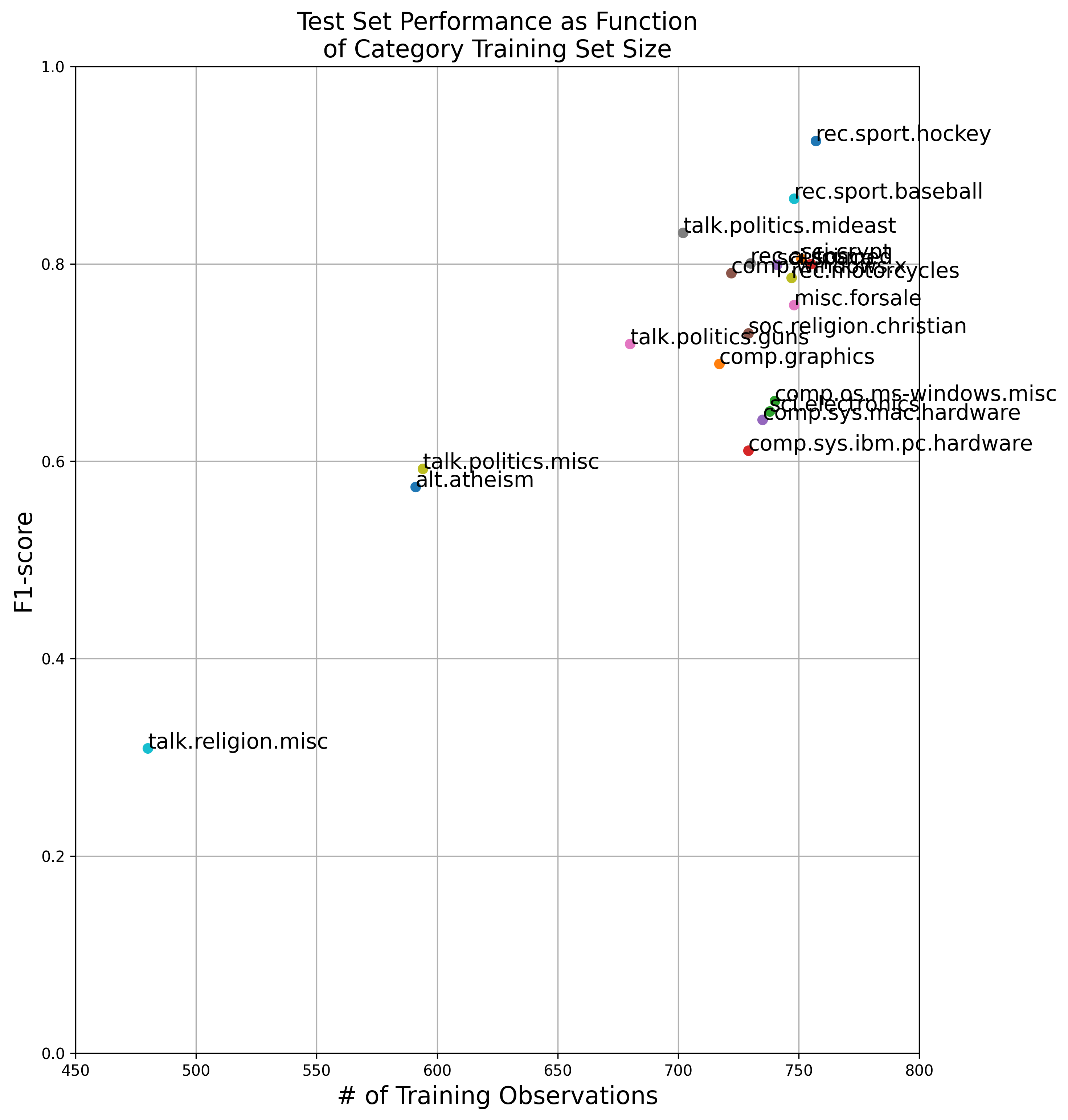
Figure 5 Performance of Simple Classifier Using Our Embeddings: blah
Python Code Used to Generate Figure 5
# Get number of training observations associates with each category
n_training_observations = Counter(y_train)
n_training_observations_per_category = {dataset.target_names[k]: n_training_observations[k] for k in n_training_observations.keys()}

# Plot relationship between Test Set F1 and # of training observations per category
plt.subplots(figsize=(10, 12), dpi=300)
for k, params in class_report.items():
    if k not in ('weighted avg', 'macro avg', 'accuracy'):
        plt.plot(n_training_observations_per_category[k], params['f1-score'], 'o')
        plt.text(n_training_observations_per_category[k], params['f1-score'], k, fontsize=14)
    plt.xlabel('# of Training Observations', fontsize=16)
    plt.ylabel('F1-score', fontsize=16)
    plt.axis('tight')
plt.xlim([450, 800])
plt.ylim([.0, 1.])
plt.title('Test Set Performance as Function\nof Category Training Set Size', fontsize=16)
plt.grid()
Figure 5 shows a roughly linear relationship between training set sample size and the testing set F1-score of the classifier. This indicates that, at least in part, sample size is a large contributor to the classifier’s performance. Further error analysis would be required to discount the first two points (beyond the scope of this post).
Wrapping Up
In this post we visited a method for calculating word embedding vectors using a classical, pre-deep-learning computational approach. Specifically we showed that with some simple frequency counts, a little information theory, and linear algebra (all methods available before the 1960s), we can derive numerical word representations that are on par with state-of-the art word embeddings that require recently-developed (well, at least since the 1980s 😉) deep learning methods.
Some benefits to this method include:
- For many out there (me included), the notion of identifying dimensions that optimize the covariance of co-occurrence statistics is way more intuitive (and less spooky/hand-wavy) than black-box models like the neural networks used in word2vec.
- SVD returns the embedding vectors in rank-order. This helps prioritize, interpret, visualize the embedding space without the need of additional PCA or t-SNE dimensionality reduction.
- No calculus required! (Not that there’s anything wrong with calculus, it’s just an extra discipline required to solve the same class of problems if using word2vec, or the like).
This is just one of the many applications that leverage the versatility of linear algebra and the Singular Value Decomposition!
Notes and References
-
O. Levy and Y. Goldberg. (2014) Neural word embedding as implicit matrix factorization. Advances in Neural Information Processing Systems (27): 2177–2185. ↩ ↩2
-
These are the eigenvalues associated with the row space of the (unscaled) covariance of PMI matrix \((PMI)^T(PMI)\). SVD applied to a symmetric matrix \(M\) returns in the left singular vectors \(U\) the eigenvectors associated with the row space of \(MM^T = M^TM\). Likewise, since the PMI matrix is symmetric, the eigenvalues returned by SVD are also associated with the covariance of the PMI matrix. ↩
-
S. Deerwester, S. T. Dumais, G. W. Furnas, T. K. Landauer, and R. Harshman. (1990). Indexing by Latent Semantic Analysis. Journal of the American Society for Information Science. 41 (6): 391–407. ↩
-
On word analogies and negative results in NLP (2019), A. Rogers ↩