p-Hacking 101: N Chasing
”\(N\) Chasing,” or adding new observations to an already-analyzed experiment can increase your experiment’s false positive rate. As an experimenter or analyst, you may have heard of the dangers of \(N\) chasing, but may not have an intuition as to why or how it increases Type I Error. In this post we’ll demonstrate \(N\) chasing using some simulations, and show that, under certain settings, adding just a single data point to your experiment can dramatically increase false positives.
Well-behaved Statistical Tests
A well-behaved statistical test should provide uniformly-distributed p-values. This is because the test shouldn’t favor any one portion of the hypothesis space over the others. This is demonstrated in Figure 1, which plots the distribution of p-values that result from running two-sample t-tests on 10,000 simulated datasets (\(N=10\)) having no difference between the two samples being tested, i.e. the Null Hypothesis \(H_0=\text{True}\).
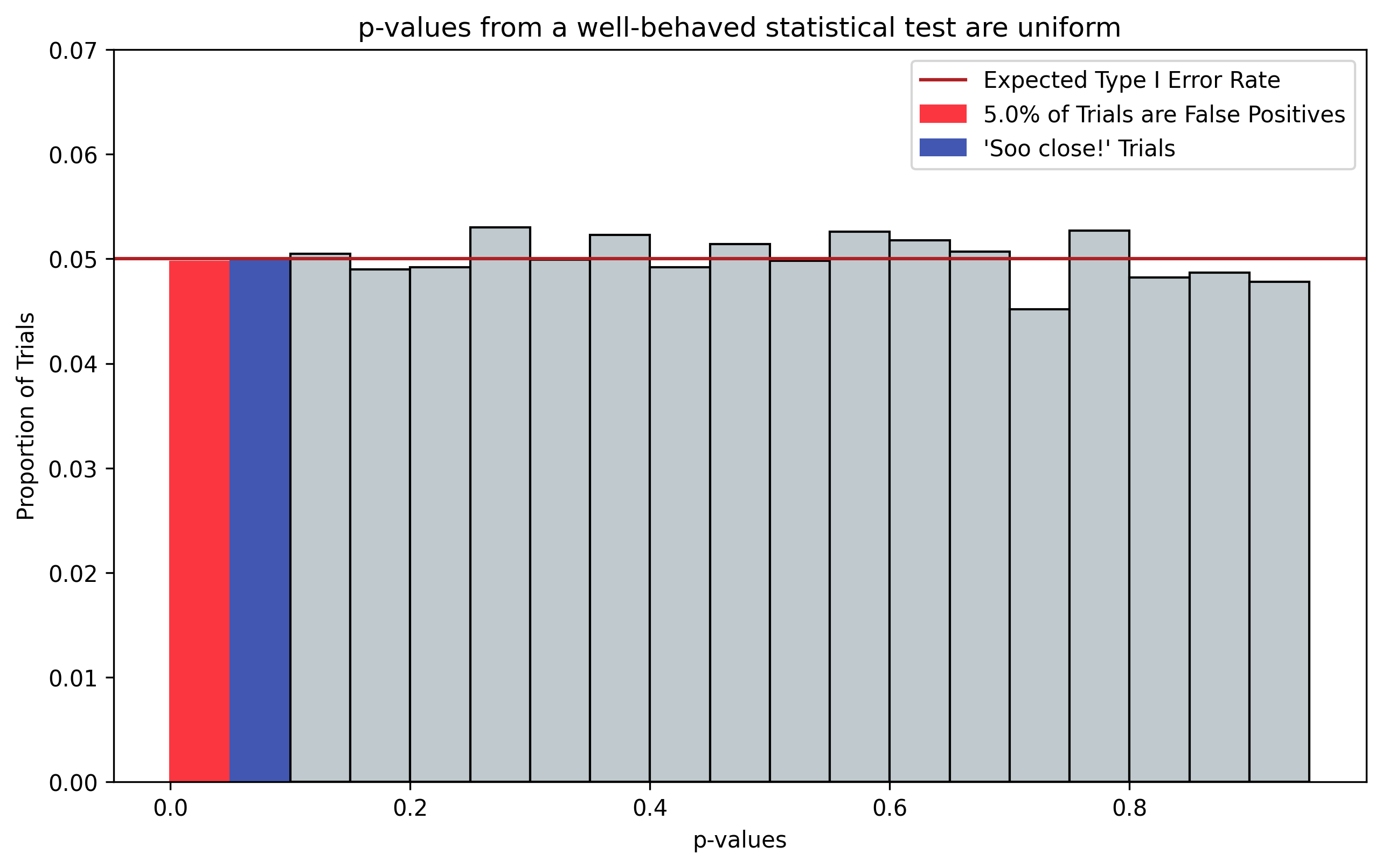
Figure 1, p-values from a well-behaved statistical test. p-values should be uniformly distributed; here we choose twenty equally-sized bins, corresponding with \(\alpha=0.05\). Even when there is no effect, i.e. \(H_0=\text{True}\), 5% of trials will indicate a “significant” effect by chance (red). Additionally, 5% of trials will be “So close” to showing significance (blue). N chasing is often performed on these “So close” trials by collecting additional data points.
Figure 1 Python Code
import numpy as np
from scipy import stats
from abra.vis import Gaussian, COLORS  # requires abracadabra
from matplotlib.patches import Rectangle

# Simulate multiple experimental datasets where H_0=True
# run t-tests, then collect the resulting p-values
ALPHA = 0.05
n_obs_per_trial, n_trials = 10, 10000
np.random.seed(1234)
null = Gaussian()
datasets = null.sample((2, n_obs_per_trial, n_trials))
pvals = stats.ttest_ind(datasets[0], datasets[1], axis=0).pvalue

def pval_rate_histogram(pvals, resolution=ALPHA, color='white', label=None):
    """Util for plotting the number of p-values that occur within buckets
    of size `resolution`.
    """
    bins = np.arange(0, 1, resolution)
    factor = 1 / float(len(pvals))
    cnts, bins = np.histogram(pvals, bins=bins)
    return plt.hist(bins[:-1], bins, weights=factor*cnts, color=color, label=label, edgecolor='black')

# Plot distribution of non-hacked p-values
plt.subplots(figsize=(10, 6))
cnt, bin_left, patches = pval_rate_histogram(pvals, color=COLORS.light_gray, label='p-values')
plt.ylim([0, .07])

# Highlight the trials bucket associated with false positives as
# well as those trials that are "Soo close" to being "significant"

## False positives trials
expected_type_I = patches[0]
expected_type_I.set_color(COLORS.red)
expected_type_I_rate = cnt[0] * 100.
expected_type_I.set_label(f"{round(expected_type_I_rate)}% of Trials are False Positives")

## So close to being "significant" trials
near_type_I = patches[1]
near_type_I.set_color(COLORS.blue)
near_type_I.set_label("'Soo close!' Trials")
plt.axhline(ALPHA, color=COLORS.dark_red, label='Expected Type I Error Rate')
plt.xlabel('p-values')
plt.ylabel('Proportion of Trials')
plt.title("p-values from a well-behaved statistical test are uniform")
plt.legend()
Because the p-vlaues are uniformly distributed, if you histogram the p-values into 20 equally-sized bins, you would expect each bin to be associated with roughly 5% of trials. Consequently, we would expect a default false positive rate \(\alpha\) of 0.05. It turns out this resolution of p-value breakdown that is a pretty common scientific standard and is one of the reasons everyone uses an \(\alpha=0.05\) in hypothesis tests.
N Chasing
Figure 1 also highlights in blue the trials where the p-values are “So close” to exhibiting a significant effect, having magnitudes just above the \(\alpha=0.05\) cutoff.
If you were an experimenter, who is incentivised to find novel, positive effects in your experiment–even though there isn’t one, as is the case here, but you don’t know that–you might be tempted to just extend your experiment juuuust a liiiiittle longer to see if the p-values for those “So close” trials decrease enough to reach statistical significance.
At first glance, adding new samples in this way seems totally reasonable. How can adding more data be bad; if the effect is there, then we should be able see it better by simply “squashing down the noise” with more samples, right? This is N chasing, a common form of p-hacking, don’t do it!
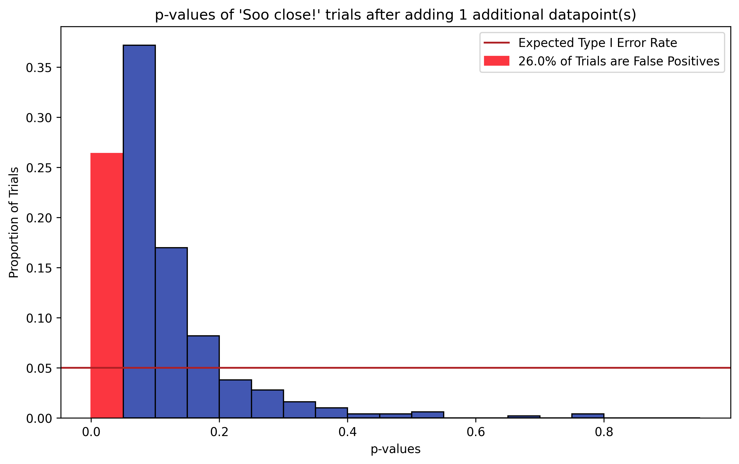
Figure 2, p-Hacking via N Chasing. To simulate N Chasing, we take the “So close” (blue) trials in Figure 1 and add to each trial a single, random data point drawn from \(H_0\) (\(N_{hacked}=11\)). The resulting distribution of p-values from running two-sample t-tests on the hacked datasets is shown. The distribution is no longer uniform–the sign of a ill-behaved statistical test. Additionally, the Type I error rate is around 25% (red bar), where we would expect false positives in around 5% of trials (dark red line).
Figure 2 Python Code
# Now hack the "So close" trials by adding samples to the H_0 dataset
## Identify the so-close trials and p-values
hack_index_mask = (pvals >= 0.05) & (pvals < .1)
hacked_datasets = datasets[:, :, hack_index_mask]
n_hacked_trials = hacked_datasets.shape[2]

## Add samples and re-run tests, collecting new p-values
n_additional_samples = 1
hacked_datasets = np.append(hacked_datasets, null.sample((2, n_additional_samples, n_hacked_trials)), axis=1)
hacked_pvals = stats.ttest_ind(hacked_datasets[0], hacked_datasets[1], axis=0).pvalue

# Display resulting hacked p-values distribution
plt.subplots(figsize=(10, 6))
hacked_cnt, hacked_bin_left, hacked_patches = pval_rate_histogram(hacked_pvals, color=COLORS.blue)
inflated_type_I = hacked_patches[0]
inflated_type_I.set_color(COLORS.red)
inflated_type_I_rate = 100. * hacked_cnt[0]
inflated_type_I.set_label(f"{round(inflated_type_I_rate)}% of Trials are False Positives")
plt.axhline(ALPHA, color=COLORS.dark_red, label='Expected Type I Error Rate')
plt.xlabel('p-values')
plt.ylabel('Proportion of Trials')

plt.legend()
plt.title(f"p-values of 'Soo close!' trials after adding {n_additional_samples} additional datapoint(s)")
To demonstrate how hacking p-values via N chasing inflates false positive rates, we take the “So close” (blue) trials from the simulation in Figure 1, and add to each trial a random data point drawn from the \(H_0\) distribution. We then re-run our two-sample t-tests and histogram the resulting p-values.
Figure 2 shows the resulting distribution of hacked p-values. These trials originally exhibited a False Positive Rate of 0% (i.e. they did not fall into the \(p \le \alpha = 0.05\) bin). However, these trials now exhibit a Type I error rate over 25% (red), nearly 5 times the expected false positive rate 5% (dark red line)! Just from adding a single data point to those trials!
Another piece of evidence suggesting that something has gone awry is that the distribution of p-values on these augmented trials is no longer uniform, but right-skewed. Thus the statistical test on these data is no longer unbiased, instead favoring lower p-values.
The problem here is that we’re adding information into the system by first calculating test statistics/p-values, interpreting the results, then deciding to add more data and testing again. It turns out that this is a flavor of statistical error known as the Multiple Comparisons Problem.1
It’s worth noting that the simulation presented here is based on a pretty small sample size of \(N=10\). Thus, adding a single data point has a much larger effect on Type I error rate than it might for larger sample sizes. However, the effect is consistent on larger \(N\) as well if one is adding new samples to the experiment that are in proportion to \(N\).
Wrapping Up
N chasing is just one of many spooky gotchas that come along with using Null hypothesis-based statistical tests (NHST). This particular p-hacking effect comes up when you know that you’ve run the experiment, did not reach significance, then decide to keep running the experiment after looking at the results. If you’ve ever said something like “oh, let’s just run it a little longer,” then you’re probably p-hacking.
The negative affects of N chasing can be minimized by sticking to standardized protocols for running experiments that use NHSTs: running an initial power analysis to calculate the required sample size for a desired effect size and statistical power, then stopping your data collection once you’ve reached the requirements prescribed by the power analysis. Continuing to collect data beyond what is prescribed will inflate your Type I error rate, and likely provide misleading results for your experiment.