Singular Value Decomposition: The Swiss Army Knife of Linear Algebra

Linear algebra provides a number powerful computational methods that are used throughout the sciences. However, I would say that hands-down the most versatile of these methods is singular value decomposition, or SVD. In this post we’ll dive into a little theory behind matrix diagonalization and show how SVD generalizes matrix diagonalization. Then we’ll go into a few of the properties of SVD and cover a few (of many!) cool and useful applications of SVD in the real world. In addition, each application will have its own dedicated post.

Matrix Diagonalization

Before introducing SVD, let’s first go over matrix diagonalization. Matrix diagonalization is the process of breaking a matrix \(M\) into two separate matrices \(P\) and \(D\), such that

\[M_{m \times m} = P_{m \times m} D_{m \times m} P_{m \times m}^{-1} \tag{1}\]

Where \(P\) is an invertible (i.e. square) matrix and \(D\) is a diagonal matrix (i.e. containing all zeros, except along the diagonal).

Now, why on earth would you want to do something like diagonalization? It turns out that representing a matrix this way has a lot of numerical and computation conveniences. For example, computing matrix inverses or matrix powers can be done efficiently for large matrices or exponents when formulated via diagonalization. Diagonalization is also often used to restate mathematical problems in a new, canonical system where certain operations or structures have convenient interpretations (e.g. finding nodes in a vibrating system or identifying energy levels in quantum mechanics).

So how does one diagonalize a matrix? There are lots of approaches to diagonalize a matrix, but a common one is to compute the eigenvalue decomposition of the matrix. To understand why this is equivalent to diagonalization, let’s note that

\[\begin{align} M &= P D P^{-1} \\ M (P) &= P D P^{-1} (P) \\ M P &= P D . \tag{2} \end{align}\]

Some of you may recognize that the statement given by Equation 2 is equivalent to finding the eigenvectors \(a_i\) and eigenvalues \(\lambda_i\) of the matrix \(M\), where

\[\begin{align} P &= \left[a_1, a_2, ... a_m\right] \\ D &= \begin{bmatrix} \lambda_1 & 0 & \dots & \dots \\ 0 & \lambda_2 & 0 & \dots \\ \vdots & \dots & \ddots & \dots \\ 0 & \dots & 0 & \lambda_m \end{bmatrix} \\ PD &= [\lambda_1 a_1, \lambda_2 a_2, ... \lambda_m a_m] \end{align}\]

Therefore solving for the eigenvalues/vectors of \(M\) provides us with the components to diagonalize \(M\) (note we’d still need to calculate the value of \(P^{-1}\)).

So what is this diagonalization operation doing, exactly? One can think of the diagonalization as performing three steps:

1. Since \(P\) is an orthonormal matrix, multiplying a vector by \(P\) (or \(P^{-1}\), depending on order of application of \(M\)) rotates the vector onto a new set of axes that are aligned with the eigenvectors of the matrix.
2. Since \(D\) is diagonal, multiplying the results of step 1 by \(D\) scales the transformed vector along each of new axes.
3. Multiplying by \(P^{-1}\) (or \(P\)) reverse rotates the rescaled vector back onto the original axes.

If all of this rotating and scaling business is still unclear, no worries, we’ll demonstrate similar ideas graphically when discussing SVD (see Figure 6).

Diagonalization isn’t for everyone: luckily there’s SVD

Looking at the diagonalization definition in Equation 1, one can infer that in order to be diagonalizable, \(M\) must be square and invertible. Although there are a lot of interesting problems that involve only square matrices there are a many, many more scenarios to do not fit this constraint. This is where SVD comes in!

One can think of SVD as a generalization of diagonalization to non-square matrices. In fact it turns out that all matrices have a SVD solution! As we’ll see, this makes SVD a more general tool than other matrix decompositions like eigenvalue decomposition, which requires square, invertible matrices.

The singular value decomposition is based on the notion that for any matrix \(M\), the matrices \(M^T M\) and \(M M^T\) are symmetric:

\[(M^T M)^T = M^T(M^T)^T = M^T M \\ (M M^T)^T = (M^T)^T M^T = M M^T\]

In addition, SVD takes advantage of the notion that all symmetric matrices like \(M^T M\) and \(M M^T\) have eigenvalues that form an orthonormal basis. With these two notion in hand, let’s first define the SVD, then we’ll derive its components from the matrices \(M^T M\) and \(M M^T\).

The singular value decomposition aims to separate an \([m \times n]\) matrix \(M\) into three distinct matrices:

\[M_{m \times n} = U_{m \times m} S_{m \times n} V_{n \times n}^T \tag{3}\]

Where \(U\) is an orthonormal matrix, \(V\) is an orthonormal matrix, and \(S\) is a diagonal matrix. To derive \(U,\) we analyze the symmetric matrix \(M^T M\) while utilizing the SVD definition of \(M\) in Equation 3:

\[\begin{align} M^T M &= (USV^T)^T(USV^T) \\ &= (VS^TU^T)(USV^T) \\ &= VS^T I S V^T \text{, since } U \text{ is orthogonal} \\ &= V S^T S V^T \\ &= V S^T S V^{-1} \text{, since } V \text{ is orthogonal} \tag{4} \end{align}\]

Look familiar? Equation 4 is essentially another diagonalization operation like the one defined in Equation 1, but this time we’re diagonalizing the matrix \(M^T M\) instead of \(M\), and have diagonalizing matrix \(S^TS\) instead of \(D\). As we showed in Equation 2, this diagonalization can be solved via eigenvalue decomposition, which suggests the two following properties of SVD:

• The columns of matrix \(V\) are simply the eigenvectors of \(M^T M\).
• Since \(S^T S\) gives the eigenvalues of \(M^T M\) along its diagonal, the diagonal of matrix \(S\) contains the square root of these eigenvalues.

OK, we’ve found \(V\) and \(S\), what about \(U\)? To derive \(U\) we perform analogous computations as for \(V\), but on \(MM^T\) instead of \(M^TM\):

\[\begin{align} MM^T &= (USV^T)(USV^T)^T \\ &= (USV^T)(VS^TU^T) \\ &= US^T I S U^T \\ &= U S^T S U^T \\ &= U S^T S U^{-1} \tag{5} \end{align}\]

Equation 5 suggests a third property of SVD, namely that the columns of \(U\) are the eigenvectors of \(M M^T.\) The matrix \(S\) has the same interpretation as in Equation 4.

Note that when \(m \neq n\), the diagonalizing matrix \(S\) is not square as was the case for \(D\) when diagonalizing square matrices. Instead \(S\) will be padded with zero rows or columns, depending on which dimension is larger. We’ll demonstrate all of this visually shortly.

Visualizing SVD

OK, we’ve written down a bunch of equations that mathematically define the components of SVD and how they related to the input matrix \(M\). Now, let’s make these derived components more tangible with some visualizations and code.

Figures 1-3 below show examples of what SVD will return for various matrix sizes. SVD and visualization code can be shown/hidden by clicking on the “▶︎ Python Code” button. Figure 1 demonstrates the results for a square matrix.

---

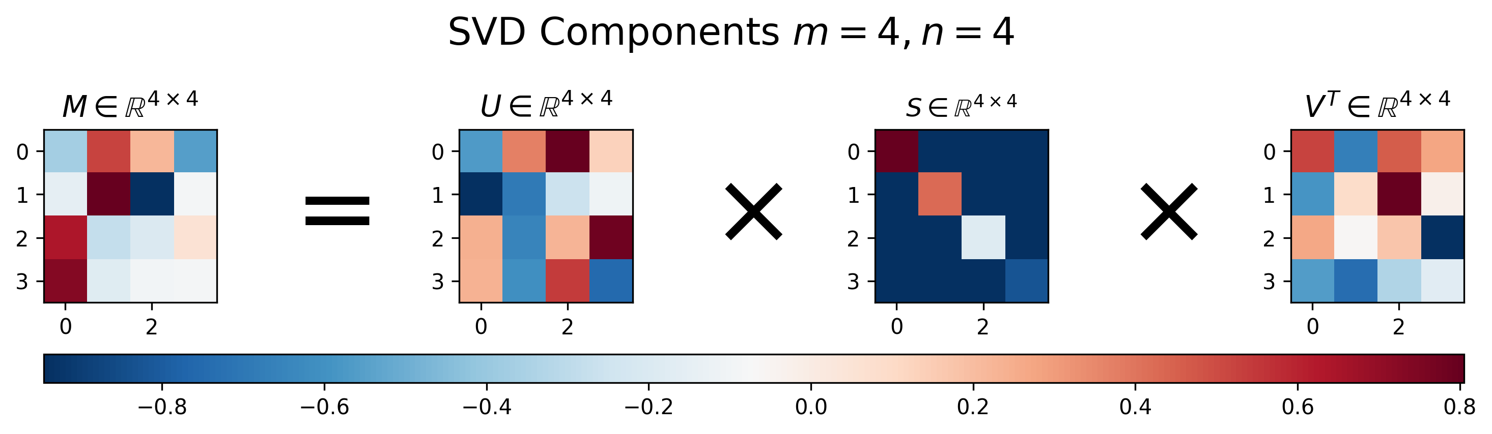
Figure 1: Visualization of \(U\), \(S\), and \(V\) for Singular Value Decomposition of a square matrix \(M\), where \(m=n\)

Python Code

import numpy as np
from matplotlib import pyplot as plt
plt.rcParams['image.cmap'] = 'RdBu_r'

PRECISION = 3


def svd(M):
    """Returns the Singular Value Decomposition of M (via Numpy), with all
    components returned in matrix format
    """
    U, s, Vt = np.linalg.svd(M)

    # Put the vector singular values into a padded matrix
    S = np.zeros(M.shape)
    np.fill_diagonal(S, s)

    # Rounding for display
    return np.round(U, PRECISION), np.round(S, PRECISION), np.round(Vt.T, PRECISION)


def visualize_svd(m, n, fig_height=5):
    """Show the Singular Value Decomposition of a random matrix of size `m x n`

    Parameters
    ----------
    m : int
        The number of rows in the random matrix
    n : int
        The number of columns
    fig_height : float
        Fiddle parameter to make figures render better (because I'm lazy and
        don't want to work out the scaling arithmetic).
    """
    # Repeatability
    np.random.seed(123)

    # Generate random matrix
    M = np.random.randn(m, n)

    # Run SVD, as defined above
    U, S, V = svd(M)

    # Visualization
    fig, axs = plt.subplots(1, 7, figsize=(12, fig_height))

    plt.sca(axs[0])
    plt.imshow(M)
    plt.title(f'$M \\in \\mathbb^{m} \\times {n}$', fontsize=14)

    plt.sca(axs[1])
    plt.text(.25, .25, '=', fontsize=48)
    plt.axis('off')

    plt.sca(axs[2])
    plt.imshow(U)
    plt.title(f'$U \\in \\mathbb{R}^{m} \\times {m}$', fontsize=14)

    plt.sca(axs[3])
    plt.text(.25, .25, '$\\times$', fontsize=48)
    plt.axis('off')

    plt.sca(axs[4])
    plt.imshow(S)
    plt.title(f'$S \\in \\mathbb{R}^{m} \\times {n}$')

    plt.sca(axs[5])
    plt.text(0.25, .25, '$\\times$', fontsize=48)
    plt.axis('off')

    plt.sca(axs[6])
    cmap = plt.imshow(V.T)
    plt.colorbar(cmap, ax=axs, orientation='horizontal', aspect=50)
    plt.title(f'$V^T \\in \\mathbb{R}^{n} \\times {n}$', fontsize=14)

    plt.suptitle(f'SVD Components $m={m}, n={n}$', fontsize=18)

    fname = f'/tmp/svd-{m}x{n}.png'
    plt.savefig(fname, bbox_inches='tight', dpi=300)
    print(fname)

visualize_svd(4, 4, fig_height=3)

---

For the square matrix, SVD returns three equally-sized square matrices. Note that unlike diagonalization defined in Equation 1, where the first and third matrices in the decomposition are the inverse of one another, for SVD this is generally not the case, i.e. \(U^{-1} \neq V^T\).

Another interesting thing to notice in Figure 1 is that the main diagonal of \(S\) has decreasing values. This is because SVD returns the singular vectors in a ranked format, where the vectors associated with largest eigenvalues are in the first columns of \(U\) and rows of \(V^T\), respectively. This turns out to be super-convenient when using SVD for applications like compression and dimensionality reduction, as you can simply choose the most “important” dimensions for the matrix representation as the first entries in the left or right singular vector matrices.

---

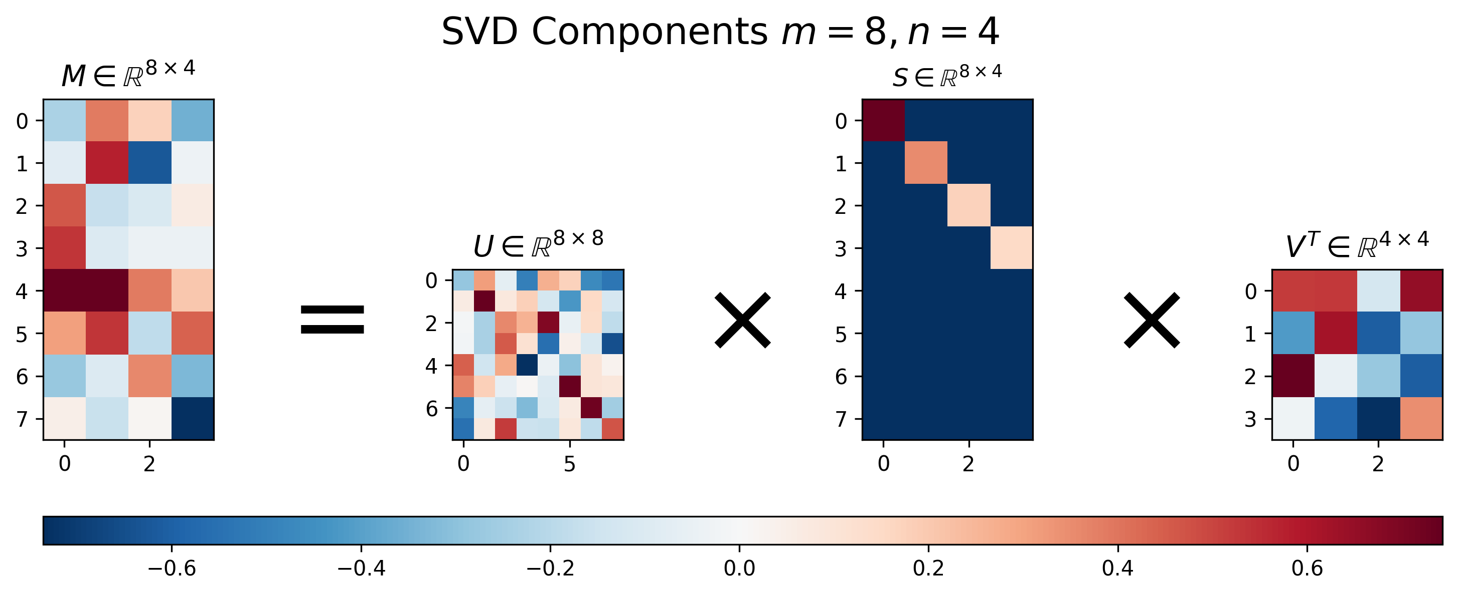
Figure 2: Visualization of \(U\), \(S\), and \(V\) for Singular Value Decomposition of a tall matrix \(M\), where \(m>n\).

Python Code

visualize_svd(8, 4, fig_height=4.5)

---

Figure 2 above shows the results of SVD applied to a “tall” matrix, where \(m > n\). We can see that the singular value matrix \(S\), though having a diagonal component with decreasing values, is no longer square. Instead it is padded with extra the rows in order to handle the extra rows in the matrix \(M\).

---

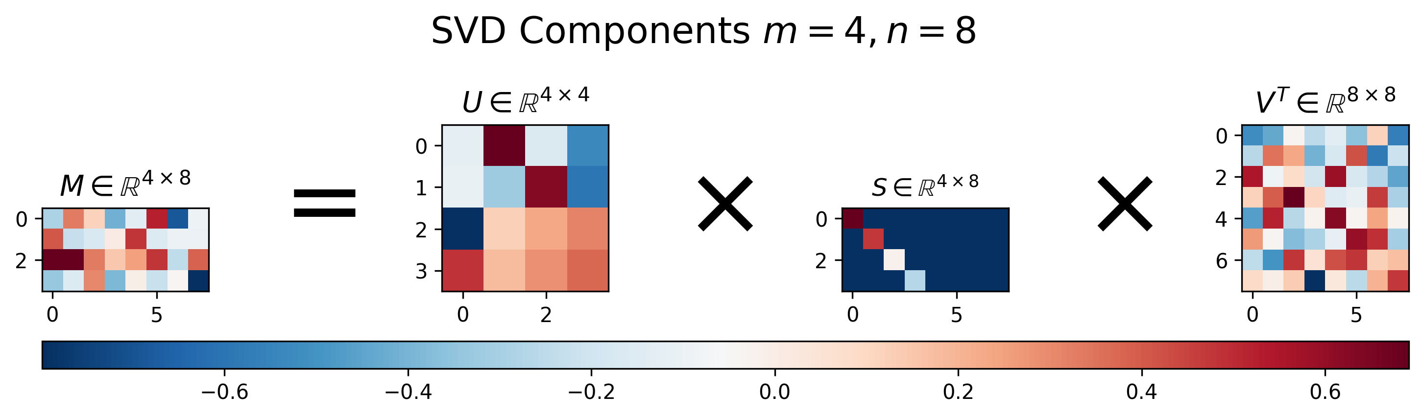
Figure 3: Visualization of \(U\), \(S\), and \(V\) for Singular Value Decomposition of a wide matrix \(M\), where \(m<n\).

Python Code

visualize_svd(4, 8, fig_height=3)

---

Figure 3 shows the results of SVD applied to a “wide” matrix, where \(m < n\). Similar to the results for the “tall” matrix, we can see that the singular value matrix \(S\) also has a diagonal component with decreasing values, but is instead padded with extra columns in order to handle the extra columns in the matrix \(M\).

Properties of SVD

The formulation of SVD ensures that the columns of \(U\) and \(V\) form an orthonormal basis. This means that all column vectors in each matrix are orthogonal/perpendicular and each vector has unit length. This is equivalent to saying that the inner product of each matrix with itself will form an identity matrix (orthogonality), and that the \(L_2\) norm of each column will be equal to one. Figure 4 below demonstrates both of these properties visually for the SVD of a matrix \(M\) with dimensionality \([10 \times 5]\).

---

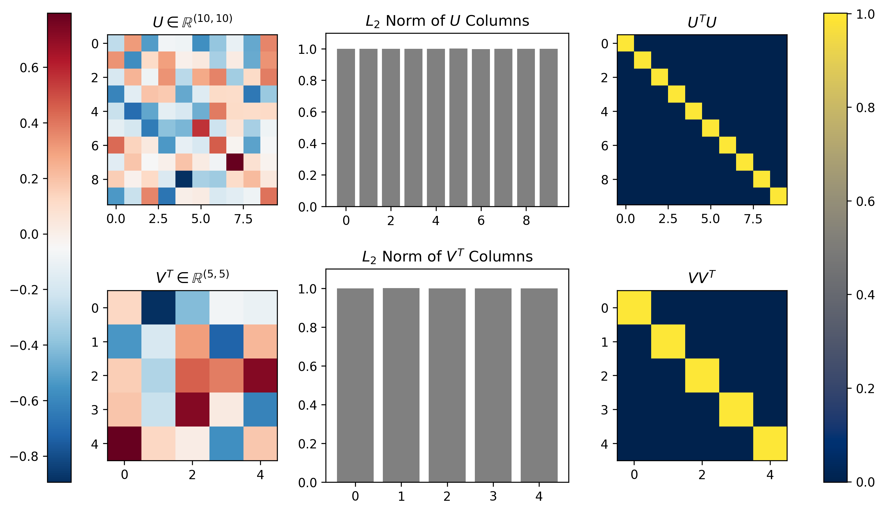
Figure 4, Singular Vectors provide an orthonormal basis: The left column shows the \(U\) and \(V^T\) that result from running SVD on a random \([m \times n] = [10 \times 5]\) matrix \(M\). The middle column plots the \(L_2\) norm calculated along the singular vectors (columns) of each matrix; the singular vectors all exhibit unit norm. The right column shows the inner product of each matrix with itself; the inner product is the identity matrix, demonstrating the orthogonality of the singular vectors.

Python Code

def matrix_column_l2_norm(M):
    """Returns the L2 norm of each column of matrix M, """
    return (M ** 2).sum(0)

# Generate random m x n matrix, M
m = 10
n = 5
np.random.seed(123)  # reproducibility
M = np.random.randn(m, n)

# Run the SVD
U, S, V = svd(M)

# Calculate L2 norm of U and V^T
U_norm = matrix_column_l2_norm(U)
V_norm = matrix_column_l2_norm(V.T)

# Visualizations
fig, axs = plt.subplots(2, 3, figsize=(12, 7))

## Matrix U
plt.sca(axs[0][0])
plt.imshow(U, interpolation='nearest')
plt.title(f'$U \in \mathbb{R}^{U.shape}$')

## L2 norm of U's columns
plt.sca(axs[0][1])
plt.gca().set_aspect(7.)
plt.bar(range(m), U_norm, facecolor='gray')
plt.ylim([0, 1.1])
plt.title('$L_2$ Norm of $U$ Columns')

## U^TU is a Identity Matrix
plt.sca(axs[0][2])
plt.imshow(U.T @ U, cmap='cividis', interpolation='nearest')
plt.title('$U^TU$')

## Matrix V
plt.sca(axs[1][0])
cax1 = plt.imshow(V.T, interpolation='nearest')
plt.title(f'$V^T \in \mathbb{R}^{V.shape}$')

## L2 norm of V^T's columns
plt.sca(axs[1][1])
plt.bar(range(n), V_norm, facecolor='gray')
plt.ylim([0, 1.1])
plt.title('$L_2$ Norm of $V^T$ Columns')

## VV^T is a Identity Matrix
plt.sca(axs[1][2])
cax2 = plt.imshow(V @ V.T, cmap='cividis', interpolation='nearest')
plt.title('$VV^T$')

## Set Colorbars
fig.colorbar(cax1, ax=[axs[0][0], axs[1][0]], location='left', pad=0.15)
fig.colorbar(cax2, ax=[axs[0][2], axs[1][2]], location='right', pad=0.15)

---

We can see that indeed the norms of all column vectors of \(U\) and \(V\) are equal to 1, and that the inner product of each indeed produces \([10 \times 10]\) and \([5 \times 5]\) identity matrices, thus indicating both matrices \(U\) and \(V\) are orthonormal basis sets.

When developing SVD above, we also established three properties relating SVD to eigenvalue decomposition:

• \(U\) contains the eigenvectors of \(MM^T\)
• \(V\) contains the eigenvectors of \(M^TM\)
• The diagonal of \(S\) contains the square root of the eigenvalues associated with \(MM^T\) and \(M^TM\)

Figure 5 below demonstrates the three properties visually for the SVD results calculated / demonstrated in Figure 4.¹

---

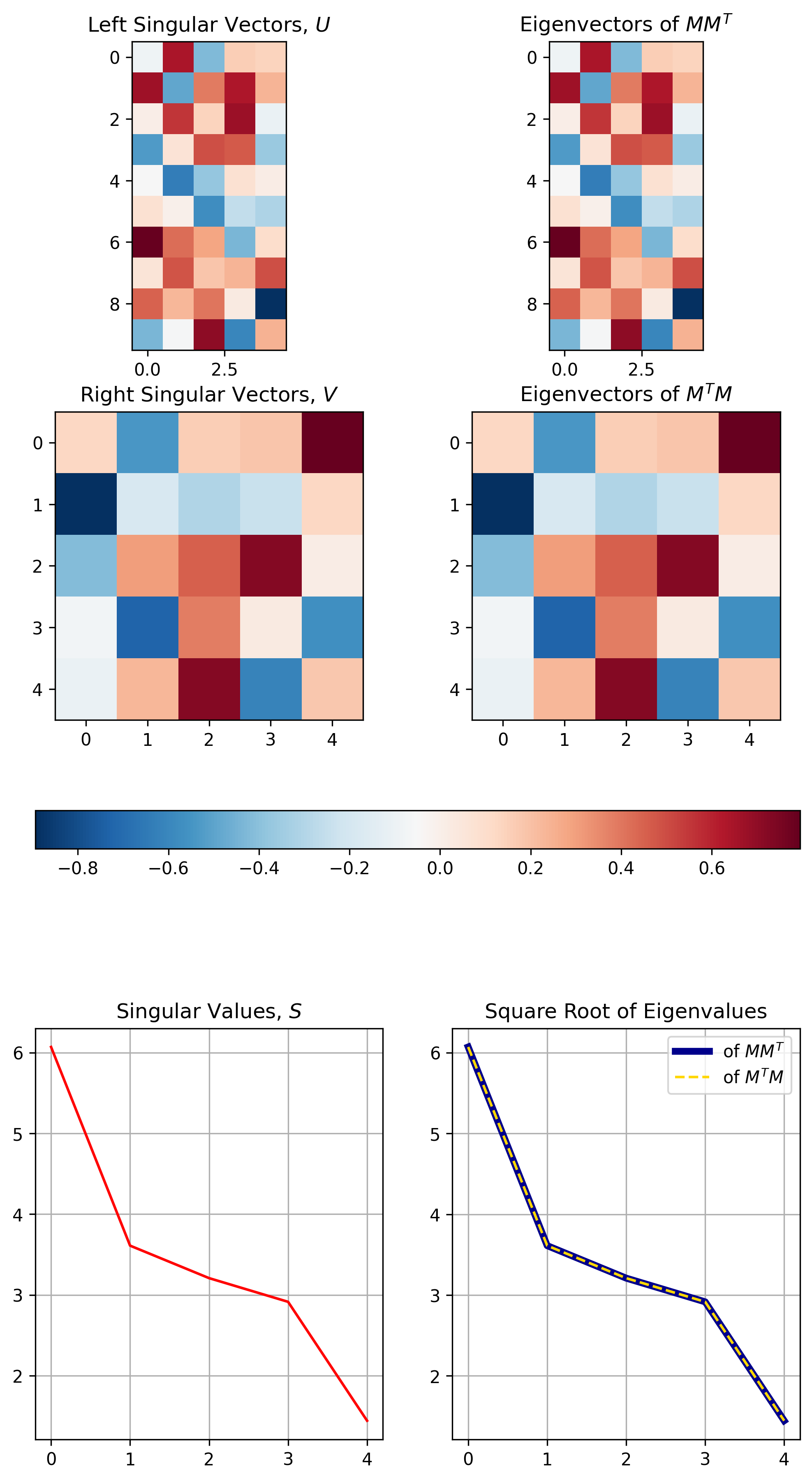
Figure 5, The relationship between SVD and Eigenvalue Decomposition: The top row demonstrates the equivalence between singular vectors \(U\) and the eigenvalues of \(MM^T\). The middle row demonstrates the equivalence between singular vectors \(V\) and the eigenvalues of \(M^TM\). The bottom row demonstrates how the singular values are equivalent to the square root of the eigenvalues of either \(MM^T\) or \(M^TM\).

Python Code

def evd(M):
    """Returns the Eigenvalue Decomposition of M (via numpy), with eigenvectors
    sorted by descending eigenvalues
    """
    def sort_eigs(evals, evecs):
        sort_idx = np.argsort(evals)[::-1]
        evals_sorted = np.round(np.real(evals[sort_idx]), PRECISION)
        evecs_sorted = np.round(np.real(evecs[:, sort_idx]), PRECISION)
        return evals_sorted, evecs_sorted

    return sort_eigs(*np.linalg.eig(M))


def align_eigen_vectors(E, M):
    """Eigenvector solutions are not unique, so check sign to give consistent results with SVD
    """
    for dim in range(E.shape[1]):
        if np.sign(M[0, dim]) != np.sign(E[0, dim]):
            E[:, dim] = E[:, dim] * -1
    return E


eigen_values_MtM, eigen_vectors_MtM = evd(M.T @ M)
eigen_values_MMt, eigen_vectors_MMt = evd(M @ M.T)

fig, axs = plt.subplots(3, 2, figsize=(8, 15))
plt.sca(axs[0][0])
# M isn't symmetric, so we only show results up to the smallest dimension, n
cax = plt.imshow(U[:, :n])
plt.title("Left Singular Vectors, $U$")

plt.sca(axs[0][1])
plt.imshow(align_eigen_vectors(eigen_vectors_MMt[:, :n], U[:, :n]))
plt.title("Eigenvectors of $MM^T$")

plt.sca(axs[1][0])
cax = plt.imshow(V)
plt.title("Right Singular Vectors, $V$")

plt.sca(axs[1][1])
plt.imshow(align_eigen_vectors(eigen_vectors_MtM, V))
plt.title("Eigenvectors of $M^TM$")
fig.colorbar(cax, ax=axs[:2], orientation='horizontal', pad=0.1)

plt.sca(axs[2][0])
plt.plot(np.diag(S), color='red')
plt.grid()
plt.title('Singular Values, $S$')

plt.sca(axs[2][1])
plt.plot(eigen_values_MMt[:n] ** .5, c='darkblue', linewidth=4, label='of $MM^T$')
plt.plot(eigen_values_MtM[:n] ** .5, '--', c='gold', label='of $M^TM$')
plt.grid()
plt.title('Square Root of Eigenvalues')
plt.legend()

---

OK, so we’ve been able to derive SVD, and visualize some of the key properties of the component matrices returned by SVD, but what is SVD actually doing? We mentioned above in the Matrix Diagonalization section that the diagonalization process is essentially a rotation, followed by a scaling, followed by a reversal of the original rotation. SVD works in a similar fashion, however, the rotations are not generally the inverses of one another.

Figure 6 provides a visual breakdown of how the transformation resulting from applying the matrix \(M\) to an input matrix of observations \(X\) can be broken down into three separate transformation operations, each provided by a component of SVD.

---

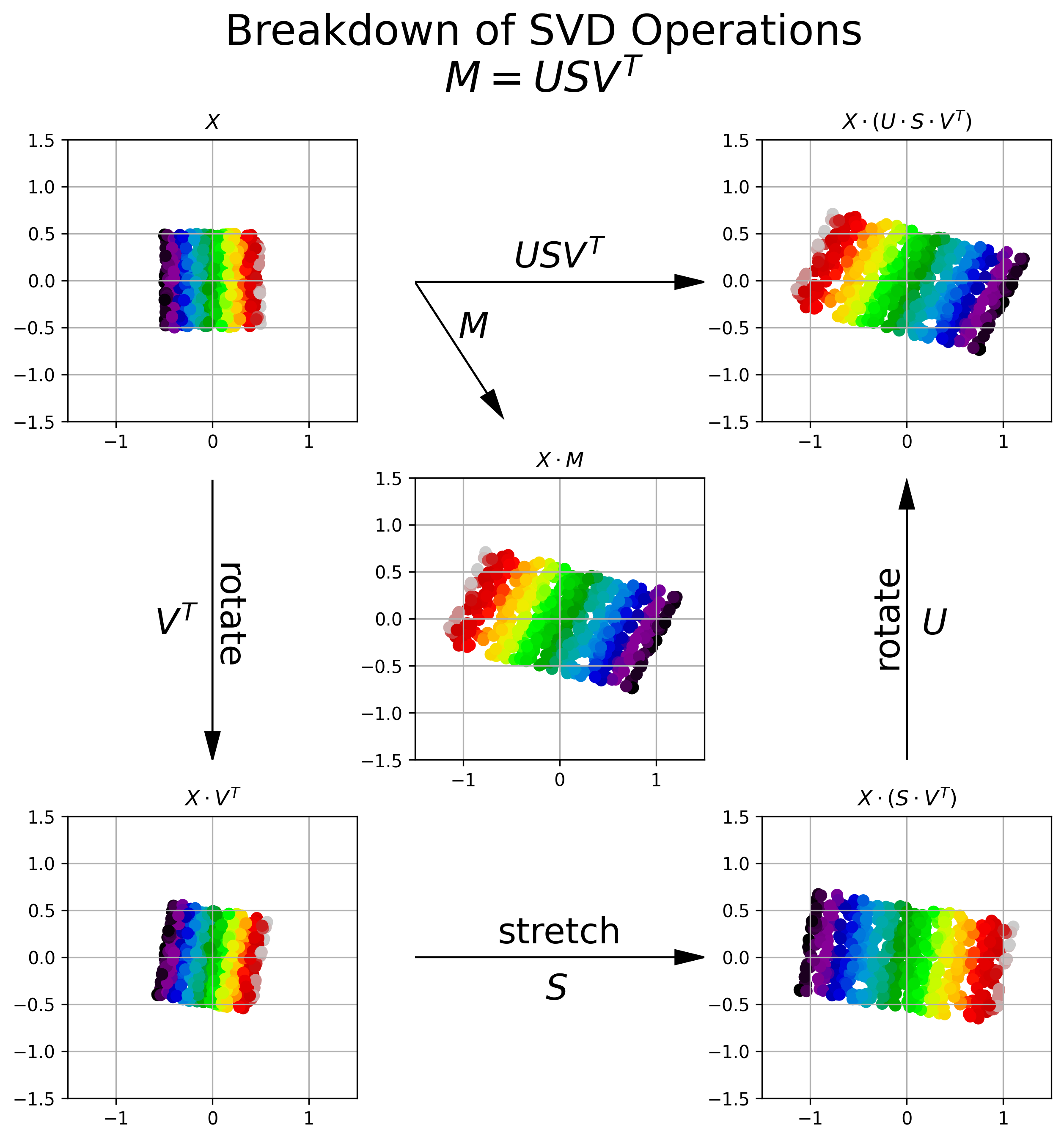
Figure 6, Visualization of SVD Operations: Upper Left: A 2D data set, distributed uniformly between \((-.5, .5)\). Each data point is colored by its relative horizontal location in the 2D coordinate system. Center: The data after being transformed by matrix \(M\). We see that \(M\) shears and flips the data about the horizontal axis. Bottom Left: The orthogonal matrix \(V^T\) rotates the original data into a new coordinate system. Bottom Right: The diagonal matrix \(S\) stretches the data along each of the primary axes in the new coordinate system. The amount of stretch is prescribed by the square root of the eigenvalues of \(M^TM\) (or alternatively \(MM^T\))). Upper Right: The orthogonal matrix \(U\) rotates the data back into the original coordinate system. We can see that the cascade of operations \(U S V^T = M\).

Python Code

# Generate random observations matrix (uniform distribution)
np.random.seed(123)  # Repeatability
n_observations = 500
n_dim = 2
X = np.random.rand(n_observations, n_dim) - .5

# Transformation Matrix
M = np.array(
    [
        [-2., .5],
        [-.5, -1]
    ]
)

colors = X[:, 0]
cmap = 'nipy_spectral'

# SVD of Transformation Matrix
U, S, V = svd(M)

# Visualization
fig, axs = plt.subplots(3, 3, figsize=(10, 10))
plt.suptitle('Breakdown of SVD Operations\n$M = U  S  V^T$', fontsize=24, ha='center')

## Data
### Original X
plt.sca(axs[0][0])
plt.scatter(X[:, 0], X[:, 1], c=colors, cmap=cmap)
plt.xlim([-1.5, 1.5])
plt.ylim([-1.5, 1.5])
plt.grid()
plt.title("$X$")

### X * M (matrix transformation)
XM = X @ M
plt.sca(axs[1][1])
plt.scatter(XM[:, 0], XM[:, 1], c=colors, cmap=cmap)
plt.xlim([-1.5, 1.5])
plt.ylim([-1.5, 1.5])
plt.grid()
plt.title("$X \cdot M$")

### X * V' (rotate)
XVt = X @ V.T
plt.sca(axs[2][0])
plt.scatter(XVt[:, 0], XVt[:, 1], c=colors, cmap=cmap)
plt.xlim([-1.5, 1.5])
plt.ylim([-1.5, 1.5])
plt.grid()
plt.title("$X \cdot V^T$")

### X * (S * V') (rotate and scale)
XSVt = X @ (S @ V.T)
plt.sca(axs[2][2])
plt.scatter(XSVt[:, 0], XSVt[:, 1], c=colors, cmap=cmap)
plt.xlim([-1.5, 1.5])
plt.ylim([-1.5, 1.5])
plt.grid()
plt.title("$X \cdot (S \cdot V^T)$")

### X * (U * S * V') (rotate, scale, and rotate)
XUSVt = X @ (U @ S @ V.T)
plt.sca(axs[0][2])
plt.scatter(XUSVt[:, 0], XUSVt[:, 1], c=colors, cmap=cmap)
plt.xlim([-1.5, 1.5])
plt.ylim([-1.5, 1.5])
plt.grid()
plt.title("$X \cdot (U \cdot S \cdot V^T)$")

## Operations/Arrows
### M
plt.sca(axs[0][1])
plt.arrow(.0, .5, .9, 0., capstyle='round', head_width=0.05, head_length=0.1, fc='black')
plt.arrow(.0, .5, .25, -.4, capstyle='round', head_width=0.05, head_length=0.1, fc='black')
plt.text(.15, .3, '$M$', fontsize=20)
plt.text(.5, .55, '$USV^T$', fontsize=20, ha='center')
plt.xlim([0., 1.])
plt.ylim([0., 1.01])
plt.axis('off')

### V'
plt.sca(axs[1][0])
plt.arrow(.5, 1., 0, -.9, capstyle='round', head_width=0.05, head_length=0.1, fc='black')
plt.text(.3, .45, '$V^T$', fontsize=20)
plt.text(.55, .35, 'rotate', fontsize=20, ha='center', rotation=-90)
plt.xlim([0., 1.])
plt.ylim([0., 1.01])
plt.axis('off')

### S
plt.sca(axs[2][1])
plt.arrow(.0, .5, .9, 0., capstyle='round', head_width=0.05, head_length=0.1, fc='black')
plt.text(.45, .35, '$S$', fontsize=20)
plt.text(.5, .55, 'stretch', fontsize=20, ha='center')
plt.xlim([0., 1.])
plt.ylim([0., 1.])
plt.axis('off')

### U
plt.sca(axs[1][2])
plt.arrow(.5, 0., 0, .9, capstyle='round', head_width=0.05, head_length=0.1, fc='black')
plt.text(.55, .45, '$U$', fontsize=20)
plt.text(.43, .35, 'rotate', fontsize=20, ha='center', rotation=90)
plt.xlim([0., 1.])
plt.ylim([0., 1.01])
plt.axis('off')

---

We can see above that SVD of matrix \(M\) breaks down the transformation encapsulated by \(M\) into a rotation (\(V^T\)), followed by a stretching (\(S\)), followed by another rotation (\(U\)).

The Swiss Army Knife of Linear Algebra

Singular Value Decomposition gives you all the theoretical, computational, and numerical benefits of diagonalization, while expanding the potential problem set to include all matrices. We’ve gone over a few distinct benefits of applying SVD, but I’ll review them and add a few others here:

• SVD can be applied to any matrix, not just invertible ones
• SVD is consistent: you get the same results each time
• SVD gives you ordered components, allowing you to “build up” a lower-dimensinal representation of \(M\) that is theoretically optimal.²
• SVD can be computed efficiently. It turns out that if you don’t require all singular vectors of the decomposition, which is almost always the case in statistics and machine learning, then you can calculate the decomposition much more efficiently, particularly if the desired rank of your approximation is small, i.e. \(r \ll m, n\).
• SVD can be computed a numerically stable fashion. Decomposing sparse matrices is often numerically unstable for decompositions methods like EVD, but SVD can easily handle sparse matrices, particularly if those matrices have low rank approximations.
• SVD provides an orthonormal basis for \(M^TM\) (through \(V^T\)) without explicitly calculating \(M^TM\). Therefore algorithms based on matrix covariance, like Principal Components Analysis, reduce to SVD.
• The matrix \(U\) gives you important/useful vectors that efficiently describe the columns of \(M\), where the rows of \(V^T\) gives you important info about the rows of \(M\). Therefore you get joint information about the column and row space of \(M\) from a single decomposition. This is not the case for eigenvalue decomposition. Having joint information about rows and columns is helpful, particularly when the rows and columns have semantic interpretations. An example would be in collaborative filtering recommendation algorithrhms that decompose a user-item preference matrix \(R\) into user-based factors (row space of \(R\)) and item-based factors (column space \(R\)).

The number of possible applications of SVD is essentially limitless. In future posts I plan to go into some details on how I use SVD to solve a number of problems in statistics, Machine Learning, NLP, and Computer Vision, including:

• Data Compression via Low-rank Approximation
• Calculating the pseudo-inverse of a non-square matrix and, related, providing the least squares solution to Linear Regression
• Providing a robust and efficient method for executing Principal Components Analysis
• Matrix completion used in recommendation systems
• Calculating robust word embedding vectors used in Natural Language Process (NLP)
• Image whitening to improve the efficieny of neural network trainig in Computer Vision
• TBD

So, I hope to see you soon for the next installment on SVD. Until then Happy Decomposing!

---

---

Resources

• Gilbert Strang’s MIT Open Courseware Course on Linear Algebra (2010)
• The Matrix Cookbook, Peterson & Pederson (2012)

Notes

1. Eigenvalue decomposition provides non-unique solutions between calculations, where the solutions may have differently ordered eigenvalues and eigenvectors can have flipped signs. Therefore to compare to SVD, which has a consistent solution, one must perform some sorting and alignment of the eigenvectors. These operations are performed in the sort_eigs and align_eigen_vectors helper functions. ↩

2. In that the rank-\(r\) approximation minimizes the Frobenius norm of the difference in actual and approximated matrix. ↩