SVD and Data Compression Using Low-rank Matrix Approximation
In a previous post we introduced the Singular Value Decomposition (SVD) and its many advantages and applications. In this post, we’ll discuss one of my favorite applications of SVD: data compression using low-rank matrix approximation (LRA). We’ll start off with a quick introduction to LRA and how it relates to data compression. Then we’ll demonstrate how SVD provides a convenient and intuitive method for image compression using a LRA.
Data Compression and Low-Rank Approximation
First off, what do we mean by low-rank approximation? Say you have an \(m \times n\) data matrix \(X\). The data contained in \(X\) could be anything, really. For example, in a computer vision setting, \(X\) could encode a single image, where each entry in the matrix is a pixel intensity value at a location encoded by the \(i,j\)-th row and column. In a machine learning setting, \(X\) could be a data set, where each row is an observation and each column is a measurable dimension. Heck, in a computer-vision-meets-machine-learning setting, \(X\) could represent multiple images, with each image being encoded as a row, and each column being one of \(n = (\text{width} \times \text{height}\)) values, encoding the image location-pixel values unraveled into a row-vector.
No matter the type of information \(X\) encodes, it will have a matrix rank \(r\), which is essentially the number of linearly independent columns (column rank) or rows (row rank) contained in the matrix. We’ll focus on column rank in this post. It’s entirely possible (and common) for a matrix to have a rank that is smaller than the number of columns in the matrix. For example, the left two plots in Figure 1 display two different matrices \(X\) and \(\tilde X\). These two matrices have the same column rank, despite having a different numbers of columns. This is because the matrix \(X\) is full rank in that its column rank is equal to the number of columns. In contrast, the matrix \(\tilde X\) contains redundant columns, resulting in a column rank that is smaller than the number of columns.1
Figure 1: Matrix Rank and Reconstruction. Left: a full-column-rank matrix \(X\). Middle: a matrix \(\tilde X\) with redundant columns formed by scaling and concatenating columns of \(X\). Right: exact reconstruction of \(\tilde X\) using a rank \(k=r=4\) singular value decomposition.
Python Code
import matplotlib.pyplot as plt
import numpy as np

plt.rcParams['image.cmap'] = 'RdBu_r'
np.random.seed(123) # Repeatability
MATRIX_RANK = 4

# Create a random matrix, which will have independent columns
# and thus a rank equal to the number of columns
X_orig = np.random.randn(8, MATRIX_RANK)
X_orig_rank = np.linalg.matrix_rank(X_orig)

# Create a new redundant matrix with twice as many columns, but new columns are
# simply a linear scaling of original matrix
X_redundant = np.hstack([-2 * X_orig, 2 * X_orig])

# Permute columns of redundant matrix
X_redundant = X_redundant[:, np.random.permutation(np.arange(X_redundant.shape[1]))]
X_redundant_rank = np.linalg.matrix_rank(X_redundant)

# Run SVD on redundant matrix, we'll use this for LRA
U, S, V = np.linalg.svd(X_redundant)

# Low-rank reconstruction (exact in this case)
X_redundant_reconstructed = U[:, :MATRIX_RANK] * S[:MATRIX_RANK] @ V[:MATRIX_RANK, :]
reconstruction_error = np.sum((X_redundant - X_redundant_reconstructed) ** 2)

# Visualizations
## Original matrix
fig, axs = plt.subplots(1, 3, figsize=(12, 5))
plt.sca(axs[0])
plt.imshow(X_orig)
plt.clim([-2, 2])
plt.title(f"A Rank $r=${X_orig_rank} matrix, X")

## Redundant matrix
plt.sca(axs[1])
plt.imshow(X_redundant)
plt.clim([-2, 2])
plt.title(f"A redundant Rank $r=${X_redundant_rank} matrix, $\\tilde X$")

## Low-rank approximation (exact reconstruction)
plt.sca(axs[2])
plt.imshow(X_redundant_reconstructed)
plt.clim([-2, 2])
plt.title(f"Reconstruction of $\\tilde X$\nusing {MATRIX_RANK} components of SVD\nTotal Squared Error: {reconstruction_error:1.1f}")
plt.suptitle("Low-Rank Approximation of a Matrix", fontsize=18)
When a matrix like \(\tilde X\) contains redundant information, that matrix can often be compressed: i.e. it can be represented using less data than the original matrix with little-to-no loss in information. One way to perform compression is by using LRA.
Low-rank approximation (Figure 2) is the process of representing the information in a matrix \(M\) using a matrix \(\hat M\) that has a rank that is smaller than the original matrix. To reduce the rank of \(\hat M\) we can attempt construct the matrix as a combination of a “tall” left-hand matrix \(L_k\) and a “wide” right-hand matrix \(R_k^T\):
\[\begin{align} M &= L R^T \\ &\approx L_k R_k^T \\ &\approx \hat M \tag{1} \end{align}\]This allows a matrix that would normally be represented using \(m \times n\) values to be represented using \(k(m + n)\) values. If \(k\) is small relative to \(m\) and \(n\), then the LRA can be used to store important information in \(M\) much more efficiently.
Figure 2: Low-rank Matrix Decomposition: A matrix \(M\) of size \(m \times n\) and rank \(r\) can be decomposed into a pair of matrices \(L_k\) and \(R_k\). When \(k=r\), the matrix \(M\) can be exactly reconstructed from the decomposition. When \(k < r\), then the decomposition provides a low-rank approximation \(\hat M\) of \(M\).
Low-rank approximation is often useful when the matrix \(M\) contains information that can be ignored, such as redundant information, or irrelevant information that isn’t helpful, or can possibly even be detrimental for solving a particular numerical problem (e.g. noise).
There are a number of methods for constructing the matrix \(\hat M\), but a common method is to use Singular Value Decomposition (SVD). Specifically, SVD decomposes matrix \(M\) into three matrices:
\[\begin{align} M &= USV^T \\ &= (US) V^T \\ &= L R^T \text{, where} \\ L &= (US) \text{, and} \\ R &= V \tag{2} \end{align}\]When full-rank SVD is used, Equation 2 provides a method to exactly reconstruct \(M\). In a similar fashion, Figure 1, right demonstrates how SVD can be used used to exactly reconstruct the redundant matrix \(\tilde X\) using a decomposition of rank \(k=r=4\), despite the matrix \(\tilde X\) having 8 columns.2
However, we’re not limited to exact reconstruction of \(M\); SVD offers a straight-forward way to obtain a low-rank approximation of \(M\). We can replace \(U\), \(S\), and \(V\) in Equation 2 with \(U_k\), \(S_k\), and \(V_k\), where we use only the first \(k\) columns of the decomposition matrices:
\[\begin{align} M &\approx U_kS_kV_k^T \\ &\approx \hat M_k. \tag{3} \end{align}\]When \(k < r\) then Equation 3 provides a LRA of \(M\), \(\hat M_k\), via SVD. We’ll demonstrate this more clearly with an example that uses SVD for image compression.
Application: Image Compression
Singular value decomposition can be used to decompose any matrix, which allows us to use SVD to compress all sorts of data, including images. Figure 3, left depicts a grayscale image, encoded as a data matrix \(X\) with rank \(r=128\). When SVD is applied to \(X\), it returns a set of left singular vectors \(U,\) right singular vectors \(V\), and a diagonal matrix \(S\) that contains the singular values associated with the singular vectors.
SVD is great because the singular vectors and values are rank-ordered in such a way that earlier components carry the most information about \(X\). The singular values in \(S\) (Figure 3, center) can be used as a proxy for the amount of information in \(X\) encoded in each component of the decomposition (Figure 3, right).
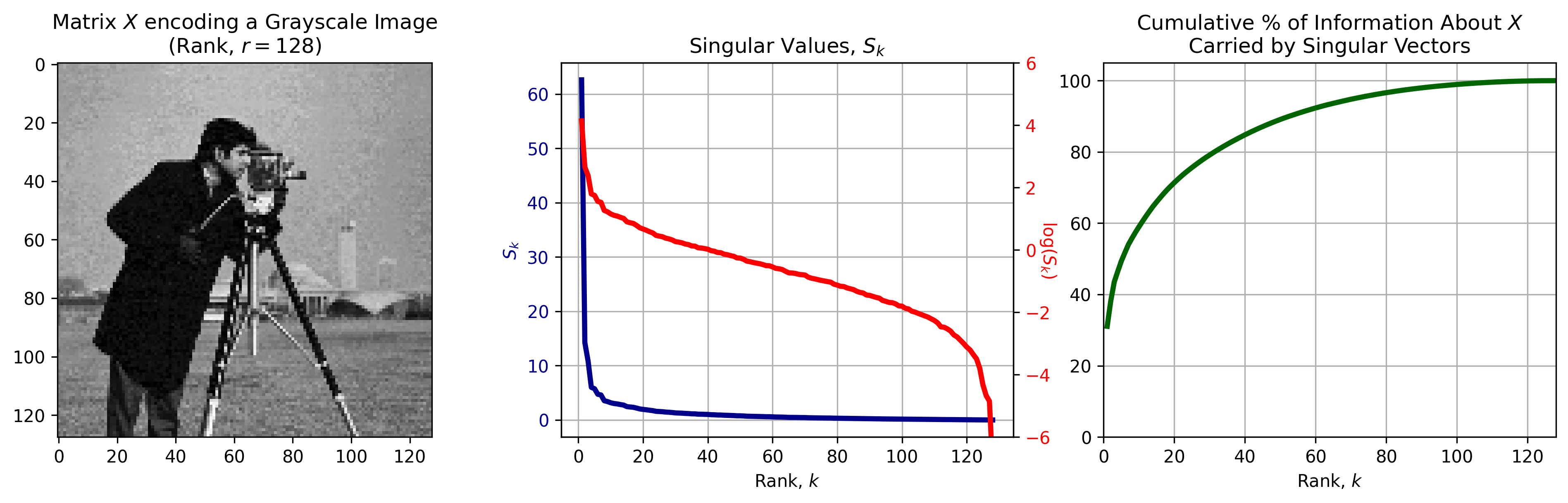
Figure 3: Singular Value Decomposition of an image \(X\). Left: A Grayscale image can be interpreted as a matrix \(X\). Center: the singular values (blue) and their log (red) as a function of rank \(k.\) Singular values decrease exponentially with rank, with earlier singular values being much larger than later ones. Right: The total information about \(X\) encoded in all the singular values up to \(k.\) A majority of information is encoded in the first singular vectors returned by SVD.
Python Code
# Load image
img = plt.imread("../assets/images/svd-data-compression/cameraman.png")

# Donwsample and encode RGBa image as matrix of intensities, X
DOWNSAMPLE = 4
R = img[::DOWNSAMPLE, ::DOWNSAMPLE, 0]
G = img[::DOWNSAMPLE, ::DOWNSAMPLE, 1]
B = img[::DOWNSAMPLE, ::DOWNSAMPLE, 2]
X = 0.2989 * R + 0.5870 * G + 0.1140 * B

# Calculate the rank of the data matrix, X
img_rank = np.linalg.matrix_rank(X, 0.)

# Run SVD on Image
U, S, V = np.linalg.svd(X)

# Calculate the cumulative variance explained by each singular value
total_S = S.sum()
n_components = len(S)
component_idx = range(1,  n_components + 1)
info_retained = 100 * np.cumsum(S) / total_S

# Visualizations
fig, axs = plt.subplots(1, 3, figsize=(16, 4))

## Raw Image, X
plt.sca(axs[0])
plt.imshow(X, cmap='gray')
plt.title(f"Matrix $X$ encoding a Grayscale Image\n(Rank, $r=${img_rank})")

## Singular values as function of rank
plt.sca(axs[1])

### Raw singular values
plt.plot(component_idx, S, label='Singular Values of $$X$$', color='darkblue', linewidth=3)
plt.grid()
plt.xlabel("Rank, $k$")
plt.ylabel('$S_k$', color='darkblue')
plt.tick_params(axis='y', labelcolor='darkblue')
plt.title('Singular Values, $S_k$')

### log(singular values)
twax = plt.gca().twinx()  # twin axes that shares the same x-axis
twax.plot(component_idx, np.log(S), color='red', linewidth=3)
plt.ylabel('$\log(S_k)$\n', color='red', rotation=270)
plt.tick_params(axis='y', labelcolor='red')
plt.ylim([-6, 6])

## Information retained as function of rank
plt.sca(axs[2])
plt.plot(component_idx, info_retained, color='darkgreen', linewidth=3)
plt.xlim(0, n_components)
plt.ylim([0, 105])
plt.xlabel("Rank, $k$")
plt.grid()
plt.title('Cumulative % of Information About $X$\nCarried by Singular Vectors')
We can see in Figure 3, center, right that a majority of the information about \(X\) is encoded in the first handfull of singular vectors/values returned by SVD. For example, 80% of information is endoded by less than a \(1/3\) of the singular vectors. This suggest that we can encode a majority of the information about the original data using only a subset of SVD components, and that it is easy to identify the optimal subset.
Figure 4 demonstrates this idea. In each row of Figure 4 we reconstruct \(X\) while increasing the rank \(k\) used in the reconstruction.3 Using only a few singular vectors (e.g. \(k=4\)) limits the reconstruction \(\hat X_k\) to encode only low-frequency spatial information about the image. As the number of singular vectors used in the approximation increases, the reconstruction includes increasing high-frequency spatial information, and thus decreasing the reconstruction error.
Using roughly 50% of the data required to store \(X\) (\(k=32)\) provides around 80% of the information in \(X,\) and the reconstruction is almost perceptually indistinguishable from the original image. We can also see that this approach isn’t a magic bullet. There’s a trade-off between the amount of data required for the reconstruction (i.e requirements for the components of \(U_k\), \(V_k\), and \(S_k\)) and the information provided about \(X\). Using 64 components results in basically no overall compression, but less than 100% information encoded. Effects like these need to be considered when using LRA for image compression.
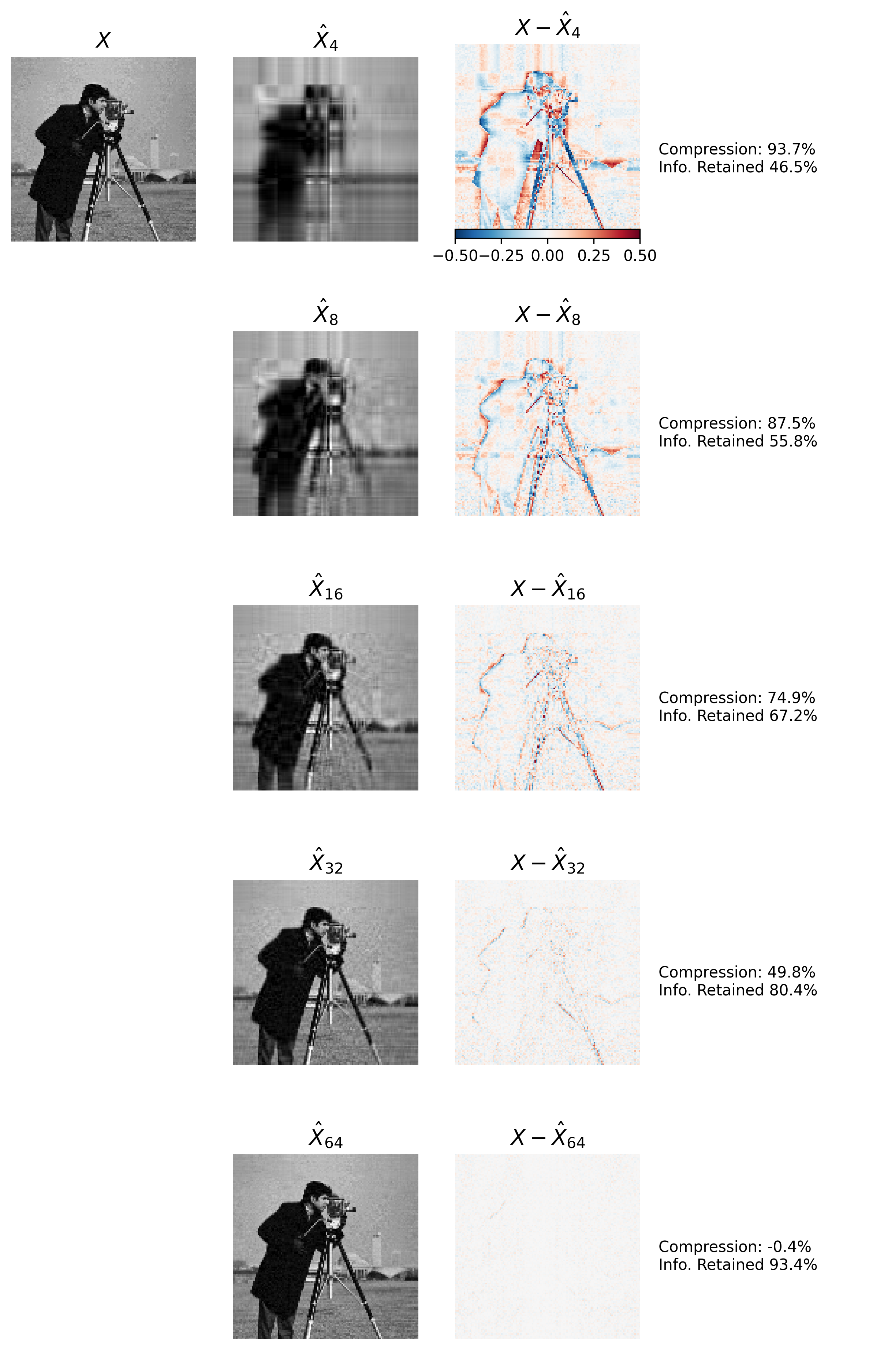
Figure 4: Image Compression via LRA/SVD. Top Left Matrix \(X\) encodes an image that we reconstruct using an increasing number of left singular vectors provided by SVD. Second Column: The approximation \(\hat{X}_k\) of image \(X\) using the first \(k\) most-informative left singular vectors. Third column: The spatial reconstruction error using approximation \(\hat{X}_k\). Right Column: displays data compression information for each row. Information includes the percentage of original image size used to represent the approximation, as well as the amount of information about \(X\) contained in the approximation.
Python Code
## Image Reconstruction
N = 5
fig, axs = plt.subplots(N, 4, figsize=(10, 16))
plt.sca(axs[0][0])
plt.imshow(X, cmap='gray')
plt.clim([0, 1.])
plt.axis('off')
plt.title("$X$", fontsize=14)

# Reconstruct image with increasing number of singular vectors/values
for power in range(1, N + 1):
    rank = 2 ** (1 + power)

    # Compressed/Reconstructed Image
    X_reconstruction = U[:, :rank] * S[:rank] @ V[:rank,:]

    # Calculate number of floats required to store compressed image
    rank_data_compression = 100 * (1. - (1. * U[:, :rank].size + S[:rank].size + V[:rank,:].size) / X.size)

    # Variance of original image explained by n components
    rank_info_retained = info_retained[rank-1]

    # Visualizations
    ## Original Image
    if power > 1:
        plt.sca(axs[power-1][0])
        plt.cla()
        plt.axis('off')

    ## Image reconstruction
    plt.sca(axs[power-1][1])
    plt.imshow(X_reconstruction, cmap='gray')
    plt.clim([0, 1.])
    plt.axis('off')
    plt.title(f'$\hat_$', fontsize=14)

    ## Reconstruction error
    plt.sca(axs[power-1][2])
    cax = plt.imshow(X - X_reconstruction)
    plt.clim([-.5, .5])
    plt.axis('off')
    plt.title(f'$X -\hat_$', fontsize=14)

    ## Compression/reconstruction info
    plt.sca(axs[power-1][3])
    compression_text = f'Compression: {rank_data_compression:1.1f}%\nInfo. Retained {rank_info_retained:1.1f}%'
    plt.text(-.1, .4, compression_text)
    plt.axis('off')

fig.colorbar(cax, ax=axs[0][2], pad=.01, orientation='horizontal')
Wrapping Up
In this post we discussed one of many applications of SVD: compression of high-dimensional data via LRA. This application is closely related to other numerical techniques such as denoising and matrix completion, as well as statistical analysis techniques for dimensionality reduction like Principal Components Analysis (PCA). Stay tuned, as I plan to dig into these additional applications of SVD in future posts. Until then, happy compressing!
Notes
-
It turns out these redundant columns have been generated by scaling and concatenating multiple columns from the full-rank matrix \(X\). ↩
-
This isn’t low-rank approximation, per se, since \(k=r\). However, it does demonstrate an important concept: redundancy can be compressed using a subset of components returned from matrix decomposition. ↩
-
In a normal compression scenario, rather than calculating the full SVD and selecting a subset of components, we would simply calculate a low-rank SVD, which can be done more efficiently than the full SVD. ↩