In this post we’ll introduce the notion of the loss function and its role in model parameter estimation. We’ll then focus in on a common loss function–the sum of squared errors (SSE) loss–and give some motivations and intuitions as to why this particular loss function works so well in practice.

Model Estimation and Loss Functions

Often times, particularly in a regression framework, we are given a set of inputs (independent variables) \(\bf{x}\) and a set outputs (dependent variables) \(\bf{y}\), and we want to devise a model function

\[f(\mathbf{x})=\mathbf{y} \tag{1}\]

that predicts the outputs given some inputs as best as possible. By “devise a model,” we generally mean estimating the parameter values of a particular model form (e.g. the weights of each term in a polynomial model, the layer weights in a neural network, etc.). But what does it mean for a model to predict “as best as possible” exactly? In order to make the notion of how good a model is explicit, it is common to adopt a loss function:

\[J(f(\mathbf{x});\mathbf{y}) \tag{2}\]

The loss function takes \(M\) input-output pairs \((x_i, y_i), i=1..M\) and returns a scalar value indicating the overall error or “loss” that results from using the model function \(f()\) to predict the outputs \(y_i\) from the associated inputs \(x_i\). “Good” models will result in a small loss values. Determining the “best” model is equivalent to finding model function that minimizes the loss function.

We generally don’t want tweak model parameters by hand, so we rely on computer programs to do the tweaking for us. There are lots of ways we can program a computer to use a loss function to identify good parameters–some examples include genetic algorithms, cuckoo search, and the MCS algorithm. However, by far the most common class of parameter optimization methods are gradient descent (GD) methods.

We won’t go deeply into GD in this post, but will point out that using GD is a process of finding optimal parameters by treating the loss function as a surface in the space of parameters, then following this surface “downhill” to the nearest location in parameter space that minimizes the loss. In order to determine the direction of “downhill”, the loss function generally needs to be differentiable at all the values that the parameters can take.

The Sum of Squared Errors Loss

Arguably, the most common loss function used in statistics and machine learning is the sum of squared of the errors (SSE) loss function:

\[\begin{align} J_{SSE}(f(\mathbf{x});\mathbf{y}) &= \sum_{i=1}^M (y_i - f(x_i))^2 \\ &= \sum_{i=1}^M e_i^2 \tag{3} \end{align}\]

This formula for \(J_{SSE}\) states that for each output predicted by the model \(f(x_i)\), we determine how “far away” the prediction is from the actual value \(y_i\). Distance is quantified by first taking the difference between the two values and squaring it. The difference between the predicted and actual value is often referred to as the model “error” or “residual” \(e_i\) for the datapoint. The semantics here being that small errors correspond to small distances. Each of the \(M\) distances are then aggregated across the entire dataset through addition, giving a single number indicating how well (or badly) the current model function captures the structure of the entire dataset. The “best” model will minimize the SSE and is called the least sum of squares (LSS) solution.

But why use this particular form of loss function in Equation 3? Why square the errors before summing them? At first, these decisions seems somewhat arbitrary. Surely there are other, more straight-forward loss functions we can devise. An initial notion of just adding the errors leads to a dead end because adding many positive and negative errors (i.e. resulting from data located below and above the model function) just cancels out; we want our measure of errors to be cumulative. Another idea would be to just take the absolute value of the errors \(\mid e_i \mid\) before summing. It turns out, this is also a common loss function, called the sum of absolute errors (SAE) or sum of absolute deviations (SAD) loss function. Though SAE/SAD is used regularly for parameter estimation, the SSE loss is generally more popular. So, why does SSE make the cut so often? It turns out there are number of interesting theoretical and practical motivations for using the SSE loss over many other losses. In the remainder of the post we’ll dig into a few of these motivations.

Geometric Interpretation and Linear Regression

One of the reasons that the SSE loss is used so often for parameter estimation is its close relationship to the formulation of one of the pillars of statistical modeling, linear regression.

Figure 1 plots a set of 2-dimensional data (blue circles). In this case the \(x_i\) encode horizontal locations and \(y_i\) the vertical locations of the (\(M=10\)) points in a 2-dimensional (2D) space. A linear function (black line) of the form

\[f_{lin}(\mathbf x) = \beta_0 + \beta_1 \mathbf x \tag{4}\]

has been fit to the data. The model parameters \(\beta_1\) (the slope of the line) and \(\beta_0\) (the offset of the line from \(y=0\)) have been optimized by minimizing the SSE loss.

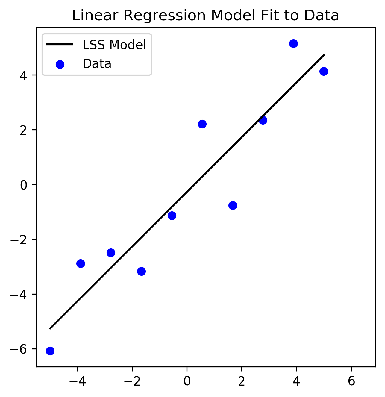
Figure 1: 2-dimensional dataset with a Linear Regression model fit. Parameters are fit by minimizing the SSE loss function

Python Code

import numpy as np
from scipy import stats
from matplotlib import patches

# Generate Dataset
np.random.seed(123)
x = np.linspace(-5, 5, 10)
y = np.random.randn(*x.shape) + x

# Find LSS solution
beta_1, beta_0, correlation_coefficient, _, _ = stats.linregress(x, y)

def linear_model_function(x):
    return beta_0 + beta_1 * x

## Plotting
DATA_COLOR = 'blue'
MODEL_COLOR = 'black'

def standardize_axis():
    plt.xlim([-7, 7])
    plt.ylim([-7, 7])
    plt.axis('square')
    plt.legend()

# Plot Data and LSS Model Fit
# fig, axs = plt.subplots(3, 1,  figsize=(20, 20))
plt.subplots(figsize=(5, 5))
# plt.sca(axs[0])
plt.scatter(x, y, color=DATA_COLOR, marker='o', label='Data')
plt.plot(x, linear_model_function(x), color=MODEL_COLOR, label='LSS Model')
standardize_axis()
plt.title('Linear Regression Model Fit to Data');

A helpful interpretation of the SSE loss function is demonstrated in Figure 2. The area of each red square is a literal geometric interpretation of each observation’s contribution to the overall loss. We see that no matter if the errors are positive or negative (i.e. actual \(y_i\) are located above or below the black line), the contribution to the loss is always an area, and therefore positive. In this interpretation, the goal of finding the LSS solution is equivalent to finding the parameters of the line that results in the smallest total red area.

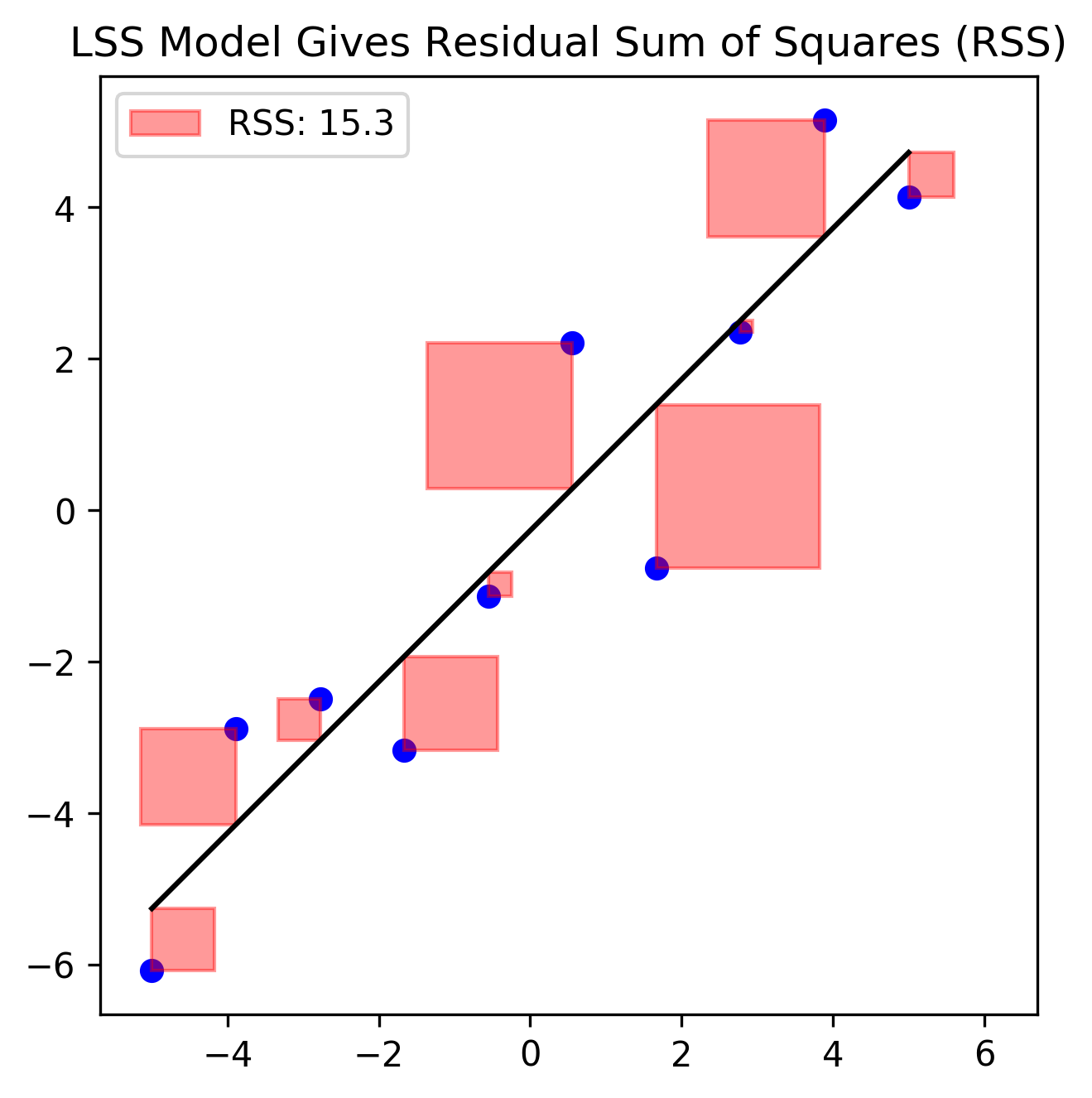
Figure 2: The SEE loss that results from the Least Squares Solution (total red area) gives the RSS; or the minimum amount of variance that cannot be explained by a linear model

Python Code

lss_loss = RSS = round(sum((y - linear_model_function(x))**2), 1)

# Plotting
LINEAR_MODEL_ERROR_COLOR = 'red'
def plot_prediction_error(x, y, prediction, color, label):
    error = y - prediction
    error_sign = np.sign(error)
    if error_sign > 0:
        bottom_left = (x - error, prediction)
    elif error_sign <= 0:
        bottom_left = (x, y)

    # error squared patch
    rect = patches.Rectangle(
        bottom_left,
        abs(error), abs(error),
        linewidth=1,
        edgecolor=color,
        facecolor=color,
        alpha=.4,
        label=label
    )
    # Add the patch to the Axes
    plt.gca().add_patch(rect)
    return rect

# Plot Least Sum of Squares Solution and RSS
plt.subplots(figsize=(5, 5))
plt.scatter(x, y, color=DATA_COLOR, marker='o')
plt.plot(x, linear_model_function(x), color=MODEL_COLOR)
plt.legend()
for data in zip(x, y, linear_model_function(x)):
    error_patch = plot_prediction_error(
        *data, color=LINEAR_MODEL_ERROR_COLOR,
        label=f"RSS: {RSS}"
    )
standardize_axis()
plt.legend(handles=[error_patch])
plt.title("LSS Model Gives Residual Sum of Squares (RSS)")

Relation to the Coefficient of Determination \(R^2\)

The geometric interpretation is also useful for understanding the important regression metric known as the coefficient of determination \(R^2\), which is an indicator of how well a linear function (i.e. Equation 4) models a dataset. First, let’s note that the variance of the model residuals takes following form:

\[\begin{align} \sigma^2_{e} &= \frac{1}{M} \sum_{i=1}^M (e_i - \mu_e)^2 \\ &= C \sum_{i=1}^M e_i^2 \\ &=C J_{SSE}(f(\mathbf{x}); \mathbf{y}) \tag{5} \end{align}\]

where we have taken the mean of the residual distribution \(\mu_e\) to be zero, as is the case in the Ordinary Least Squares (OLS) formulation. Therefore, we can think of the SSE loss as the (unscaled) variance of the model errors. Therefore minimizing the SEE loss is equivalent to minimizing the variance of the model residuals. For this reason, the sum of squares loss is often referred to as the Residual Sum of Squares error (RSS) for linear models.

Now, imagine that instead of modeling the data with the full linear model depicted in Figures 1-2, we instead us a simpler model that has no slope parameter, and only a bias/offset parameter (i.e. \(\beta_0\)). In this case the simpler model, shown in Figure 3, only captures the mean value of the data along the y-dimension.

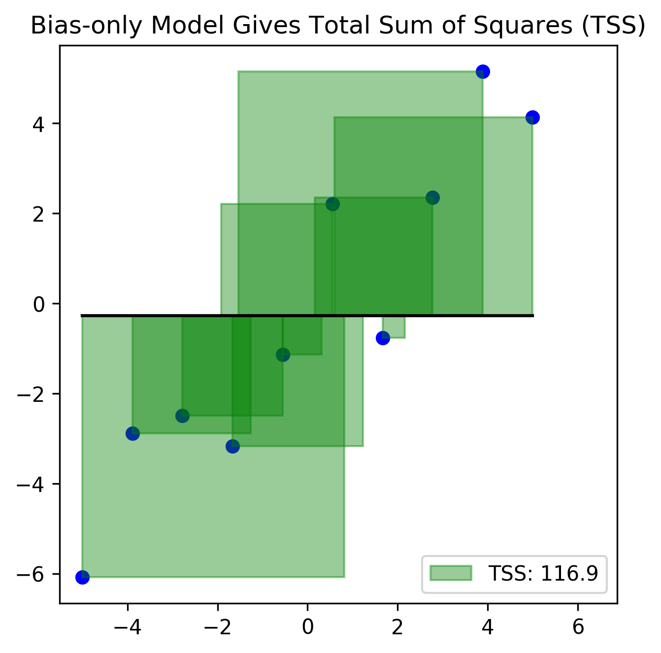
Figure 3: The SSE loss that results from a bias-only model (total green area) gives the TSS, which can be thought of as the (unscaled) variance of the data set’s output variables

Python Code

# offset parameter of LSS solution is the mean of outputs
assert y.mean() == beta_0

def bias_only_model(x):
    return beta_0 * np.ones_like(x)

bias_only_loss = TSS = round(sum((y - bias_only_model(x))**2), 1)

# Plotting
BIAS_ONLY_MODEL_COLOR = 'green'

# Bias-only Model Solution gives TSS
plt.subplots(figsize=(5, 5))
plt.scatter(x, y, color=DATA_COLOR, marker='o', label='Data')
plt.plot(x, bias_only_model(x), color=MODEL_COLOR, label='LSS')
for data in zip(x, y, bias_only_model(x)):
    error_patch = plot_prediction_error(
        *data,
        color=BIAS_ONLY_MODEL_COLOR,
        label=f"TSS: {TSS}"
    )
standardize_axis_dims()
plt.legend(handles=[error_patch])
plt.title("Bias-only Model Gives Total Sum of Squares (TSS)")

The total squared error in this model corresponds to the (unscaled) variance of the data set itself, and is often referred to as the the Total Sum of Squares (TSS) error.

The metric \(R^2\) is defined from the RSS and TSS (total red and green areas, respectively) as follows:

\[R^2 = 1 - \frac{RSS}{TSS} \tag{5}\]

If the linear model is doing a good job of fitting the data, then the variance of the model errors (RSS, red area) will be small compared to the variance of the dataset (TSS, green area), and the \(R^2 \rightarrow 1\). If the model is doing a poor job of fitting the data, then the variance residuals will approach that of the data itself, and \(R^2\) will be close to zero¹. This is why the \(R^2\) metric is often used to describe “the amount of variance in the data accounted for by the linear model.”

Relation to the correlation coefficient, Pearson’s \(r\)

During the model fitting using scipy.stats.linregress, we made sure to assign the correlation_coefficient variable returned from the optimization procedure. This is Pearson’s \(r\) correlation coefficient (CC), and is defined as the covariance between two random variables (i.e. two equal-length arrays of numbers) \(A, B\), rescaled by the product of each variable’s standard deviation:

\[r = \frac{\text{Cov}(A, B)}{\sigma_A \sigma_B} \tag{6}\]

In the case of linear regression, \(A=\mathbf y\) and \(B=f(\mathbb{x})\). In this scenario, it turns out that \(r = \sqrt{R^2}\). Therefore if we calculate \(\sqrt{1 - \frac{RSS}{TSS}}\), we should recover the correlation coefficient. We verify this notion with the results of our simulation in three ways:

Calculating CC from the \(R^2\) derived from the SSE loss function
Calculating the CC from raw data and predictions
Verifying the CC returned by the scipy fitting procedure

Python Code

lss_loss = RSS = round(sum((y - linear_model_function(x))**2), 1)
bias_only_loss = TSS = round(sum((y - bias_only_model(x))**2), 1)
r_squared = 1 - RSS / TSS
r = np.sqrt(r_squared)
raw_cc = np.corrcoef(y, linear_model_function(x))[0][1]

print(r"0. R^2 derived from loss functions: {:1.3f}".format(r_squared))
print(f"1. Correlation derived from R^2: {r:1.3f}")
print(f"2. Raw correlation (numpy): {raw_cc:1.3f}")
print(f"3. Correlation returned by model fit: {correlation_coefficient:1.3f}")

# 0. R^2 derived from loss functions: 0.869
# 1. Correlation derived from R^2: 0.932
# 2. Raw correlation (numpy): 0.932
# 3. Correlation returned by model fit: 0.932

We can see that we’re able to recover the CC from our loss function values RSS and TSS. Therefore we can think of minimizing the SSE loss as maximizing the covariance between the real outputs and those predicted by the model.

Physical Interpretation & Variable Covariance

We can gain some additional insight to the importance of minimizing the SSE loss by developing concepts within the framework of a physical system, depicted in Figure 4. In this formulation, a set of springs (red, dashed lines, our errors \(e_i\)) suspend a bar (black line, our linear function \(f(\mathbf{x})\)) to a set of anchors (blue datapoints, our outputs \(\mathbf{y}\)). Note that in this formulation, the springs are constrained to operate only along the vertical direction (\(y\)-dimension). This constraint is equivalent to saying that there is only error in our measurement of the dependent variables, and is often an assumption made in regression frameworks.

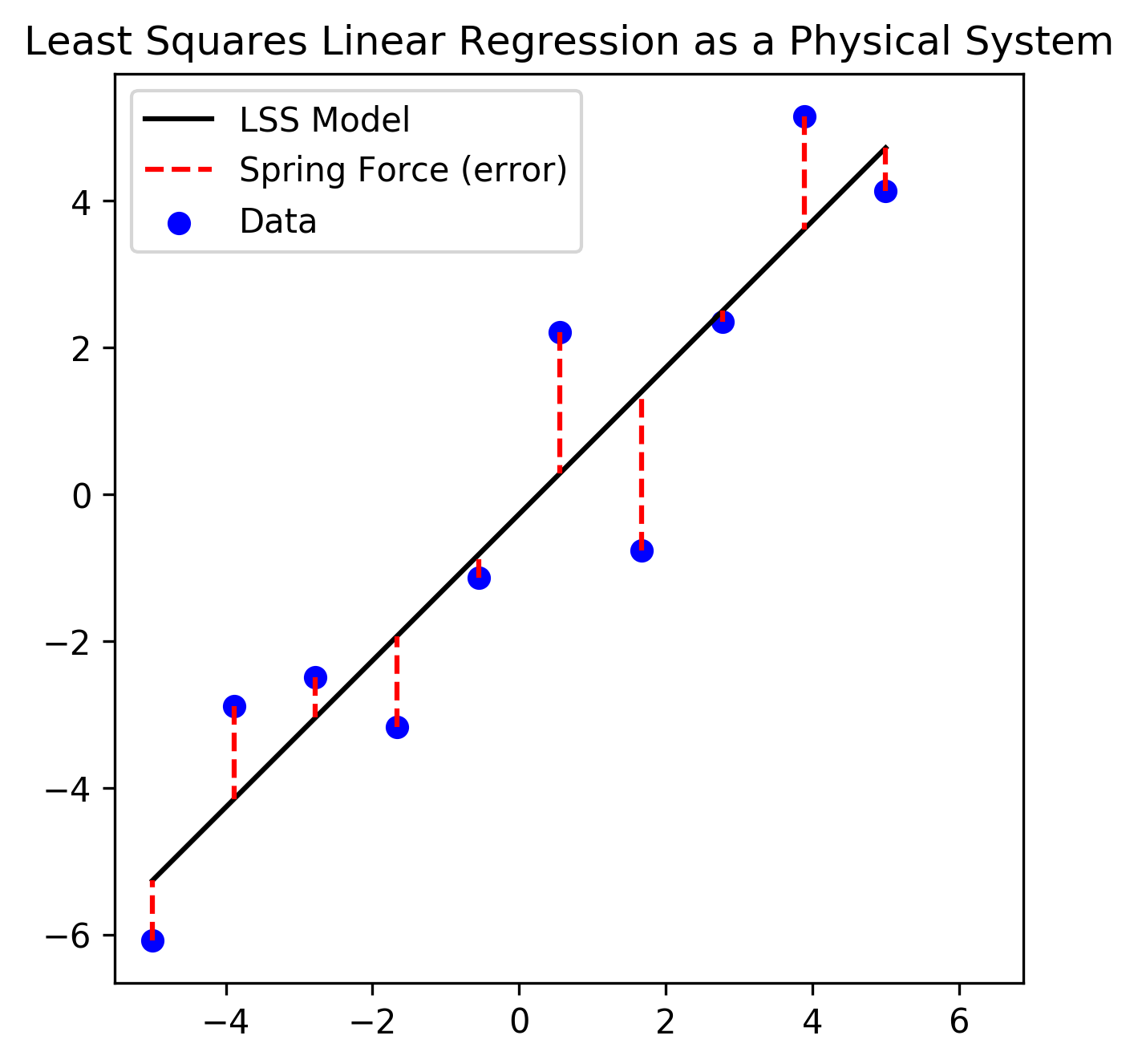
Figure 4: Modeling linear regression as a physical system of a bar (linear model function \(f(\mathbf x)\)) suspended by the force of multiple springs (model errors \(\mathbf e\))

Python Code

# Plot Error as physical system
plt.subplots(figsize=(5, 5))
plot_data_and_linear_model()

def plot_springs():
    for ii, (x_, y_, pred) in enumerate(zip(x, y, linear_model_function(x))):
        label = None if ii > 0 else "Spring Force (error)"
        plt.plot((x_, x_), (y_, pred), 'r--', label=label)
    plt.legend()
        
plot_springs()
plt.title('Least Squares Linear Regression as a Physical System')

From Hooke’s Law, the force created by each spring on the bar is proportional to the distance (error) from the bar (linear function) to its corresponding anchor (data point):

\[F_i = -ke_i\]

Further, there is a potential energy \(U_i\) associated with each spring (datapoint). The total potential energy for the system is defined as:

\[\begin{align} \sum_i U_i &= \sum_i \int -k e_i \text{d}e_i \\ &= \sum_i \frac{1}{2} k e_i^2 \\ &= \sum_i (y_i - f(x_i))^2 \end{align}\]

(assuming a spring constant of \(k=2\)). This demonstrates that the equilibrium state of this system (i.e. the arrangement of the bar that minimizes the potential energy of the system) is analogous to the state that minimizes the sum of the squared error (distance) between the bar (linear function) and the anchors (data points).

The physical interpretation can also be used to derive how linear regression solutions are related to the variances of the independent variables \(\mathbf x\) and the covariance between \(\mathbf x\) and \(\mathbf y\). When the bar is in the equilibrium position, the net force exerted on the bar is zero. Because \(\mathbf{\hat y} = \beta_0 + \beta_1 \mathbf x\), this first zero-net-force condition is formally described as:

\[\sum_i^M y_i - \beta_0 - \beta_1x_i = 0\]

A second condition that is fulfilled during equilibrium is that there are no torquing forces on the bar (i.e. the bar is not rotating about an axis). Because torque created about an axis is the force times distance away from the origin (average \(x\)-value; the origin), this second zero-net-torque condition is formally described by:

\[\sum_i^M x_i(y_i - \beta_0 - \beta_1 x_i) = 0\]

From the equation corresponding to the first zero-net-force condition², we can solve for the bias parameter \(\beta_0\) of the linear function that describes the orientation of the bar:

\[\begin{align} \beta_0 &=\frac{1}{M}\sum_i (y_i - \beta_1 x_i) \\ &= \bar y - \beta_1 \bar x \end{align}\]

Here the \(\bar \cdot\) (pronounced “bar”) means the average value. Plugging this expression into the second second zero-net-torque condition equation, we discover that the slope of the line has an interesting interpretation related to the variances of the data:

\[\begin{align} \sum_i x_i(y_i - \beta_0 - \beta_1x_i) &= 0 \\ \sum_i x_i(y_i - (\bar y - \beta_1 \bar x) - \beta_1x_i) &= 0 \\ \sum_i x_i(y_i - \bar y) &= \beta_1 \sum_i x_i(x_i - \bar x) \\ \sum_i (x_i - \bar x)(y_i - \bar y) &= \beta_1 \sum_i (x_i -\bar x)^2 \\ \beta_1 = \frac{\sum_i (x_i - \bar x)(y_i - \bar y)}{\sum_i (x_i -\bar x)^2} &= \frac{\text{cov}(x,y)}{\text{var}(x)} \end{align}\]

The expressions for the parameters \(\beta_0\) and \(\beta_1\) tell us that under least squares linear regression the average of the dependent variables is equal to a scaled version of the average of independent variables plus an offset \(\beta_0\):

\[\bar y = \beta_0 + \beta_1 \bar x\]

Further, the scaling factor \(\beta_1\) (the slope) is equal to the ratio of the covariance between the dependent and independent variables to the variance of the independent variable. Therefore if \(\mathbf x\) and \(\mathbf y\) are positively correlated, the slope will be positive, if they are negatively correlated, the slope will be negative.

Therefore, the SSE loss function directly relates model residuals to how the independent and dependent variables co-vary. These formal covariance-flavored relationships are not available with other loss functions such as the least absolute deviation.

Because of these relationships, the LSS solution has a number of useful properties:

The sum of the residuals under the LSS solution is zero (this is equivalent to the zero-net-force condition).
Because of 1., the average residual of the LSS solution is zero (this was also pointed out in the geometric interpretation above)
The covariance between the independent variables and the residuals is zero (because the residual term in OLS \(\epsilon \sim N(0, I)\) is \(\text{i.i.d.}\)).
The LSS solution minimizes the variance of the residuals/model errors (also pointed out in the geometric interpretation).
The LSS solution always passes through the mean (center of mass) of the sample.

Wrapping up

Though not covered in this post, there are many other motivations for using the SSE loss over other loss functions, including (but not limited to):

The Least Squares solution can be derived in closed form, allowing simple analytic implementations and fast computation of model parameters.
Unlike the LAE loss, the SSE loss is differentiable (i.e. it is smooth) everywhere, which allows model parameters to be estimated using straight-forward, gradient-based optimizations
Squared errors have deep ties in statistics and maximum likelihood estimation methods (as mentioned above), particularly when the errors are distributed according the Normal distribution (as is the case in the OLS formulation)
There are a number of geometric and linear algebra theorems that support using least squares. For instance the Gauss-Markov theorem states that if errors of a linear function are distributed Normally about the mean of the line, then the LSS solution gives the best unbiased estimator for the parameters \(\mathbf \beta\).
Squared functions have a long history of facilitating calculus calculations used throughout the physical sciences. The SSE loss does have a number of downfalls as well. For instance, because each error is squared, any outliers in the dataset can dominate the parameter estimation process. For this reason, the LSS loss is said to lack robustness. Therefore preprocessing of the the dataset (i.e. removing or thresholding outlier values) may be necessary when using the LSS loss.

Notes

Note too that the value of R\(^2\) can take negative values, in the case when the RSS is larger than the TSS, indicating a very poor model. ↩
What’s interesting, is that the two physical constraint equations derived from the physical system are also obtained through other analytic analyses of linear regression including defining the LSS problem using both maximum likelihood estimation and the method of moments. ↩