Derivation: Derivatives for Common Neural Network Activation Functions
When constructing Artificial Neural Network (ANN) models, one of the primary considerations is choosing activation functions for hidden and output layers that are differentiable. This is because calculating the backpropagated error signal that is used to determine ANN parameter updates requires the gradient of the activation function gradient . Three of the most commonly-used activation functions used in ANNs are the identity function, the logistic sigmoid function, and the hyperbolic tangent function. Examples of these functions and their associated gradients (derivatives in 1D) are plotted in Figure 1.
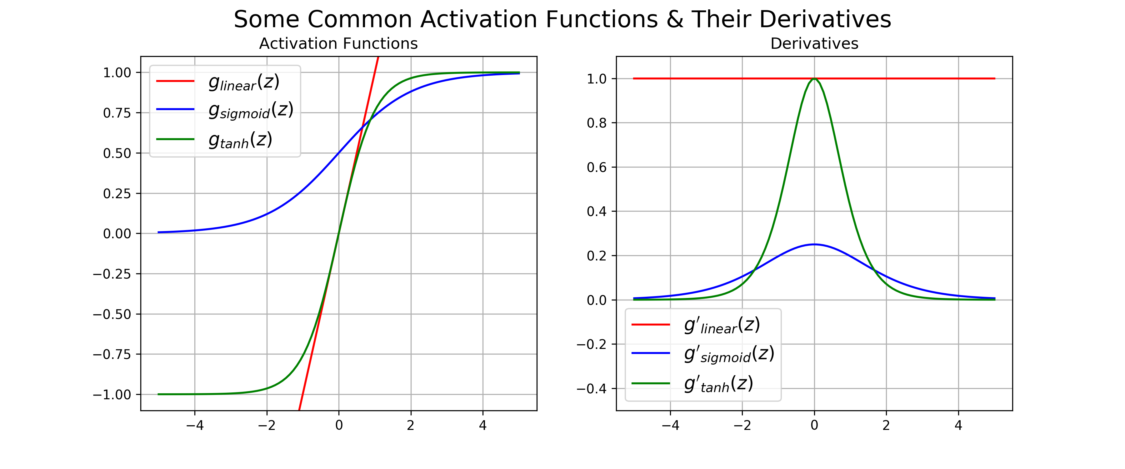
Figure 1: Common activation functions functions used in artificial neural, along with their derivatives
In the remainder of this post, we derive the derivatives/gradients for each of these common activation functions.
The Identity Activation Function
The simplest activation function, one that is commonly used for the output layer activation function in regression problems, is the identity/linear activation function (Figure 1, red curves):
\[g_{linear}(z) = z\]This activation function simply maps the pre-activation to itself and can output values that range \((-\infty, \infty)\). Why would one want to do use an identity activation function? After all, a multi-layered network with linear activations at each layer can be equally-formulated as a single-layered linear network. It turns out that the identity activation function is surprisingly useful. For example, a multi-layer network that has nonlinear activation functions amongst the hidden units and an output layer that uses the identity activation function implements a powerful form of nonlinear regression. Specifically, the network can predict continuous target values using a linear combination of signals that arise from one or more layers of nonlinear transformations of the input.
The derivative of \(g_{\text{linear}}\) , \(g'_{\text{linear}}\), is simply 1, in the case of 1D inputs. For vector inputs of length D the gradient is \(\vec{1}^{1 \times D}\), a vector of ones of length D.
The Logistic Sigmoid Activation Function
Another function that is often used as the output activation function for binary classification problems (i.e. outputs values that range (0, 1)), is the logistic sigmoid (Figure 1, blue curves). The logistic sigmoid has the following form:
\[\begin{array}{rcl} g_{\text{logistic}}(z) = \frac{1}{1 + e^{-z}}\end{array}\]and outputs values that range (0, 1). The logistic sigmoid is motivated somewhat by biological neurons and can be interpreted as the probability of an artificial neuron “firing” given its inputs. (It turns out that the logistic sigmoid can also be derived as the maximum likelihood solution to for logistic regression in statistics). Calculating the derivative of the logistic sigmoid function makes use of the quotient rule and a clever trick that both adds and subtracts a one from the numerator:
\[\begin{array}{rcl} g'_{\text{logistic}}(z) &=& \frac{\partial}{\partial z} \left ( \frac{1}{1 + e^{-z}}\right ) \\ &=& \frac{e^{-z}}{(1 + e^{-z})^2} \text{(by chain rule)} \\ &=& \frac{1 + e^{-z} - 1}{(1 + e^{-z})^2} \\ &=& \frac{1 + e^{-z}}{(1 + e^{-z})^2} - \left ( \frac{1}{1+e^{-z}} \right )^2 \\ &=& \frac{1}{(1 + e^{-z})} - \left ( \frac{1}{1+e^{-z}} \right )^2 \\ &=& g_{\text{logistic}}(z)- g_{\text{logistic}}(z)^2 \\ &=& g_{\text{logistic}}(z)(1 - g_{\text{logistic}}(z)) \end{array}\]Here we see that \(g'_{logistic}(z)\) evaluated at \(z\) is simply \(g_{logistic}(z)\) weighted by \((1-g_{logistic}(z))\). This turns out to be a convenient form for efficiently calculating gradients used in neural networks: if one keeps in memory the feed-forward activations of the logistic function for a given layer, the gradients for that layer can be evaluated using simple multiplication and subtraction rather than performing any re-evaluating the sigmoid function, which requires extra exponentiation.
The Hyperbolic Tangent Activation Function
Though the logistic sigmoid has a nice biological interpretation, it turns out that the logistic sigmoid can cause a neural network to get “stuck” during training. This is due in part to the fact that if a strongly-negative input is provided to the logistic sigmoid, it outputs values very near zero. Since neural networks use the feed-forward activations to calculate parameter gradients (again, see this this post for details), this can result in model parameters that are updated less regularly than we would like, and are thus “stuck” in their current state.
An alternative to the logistic sigmoid is the hyperbolic tangent, or \(\text{tanh}\) function (Figure 1, green curves):
\[\begin{array}{rcl} g_{\text{tanh}}(z) &=& \frac{\text{sinh}(z)}{\text{cosh}(z)} \\ &=& \frac{\mathrm{e}^z - \mathrm{e}^{-z}}{\mathrm{e}^z + \mathrm{e}^{-z}}\end{array}\]Like the logistic sigmoid, the tanh function is also sigmoidal (“s”-shaped), but instead outputs values that range \((-1, 1)\). Thus strongly negative inputs to the tanh will map to negative outputs. Additionally, only zero-valued inputs are mapped to near-zero outputs. These properties make the network less likely to get “stuck” during training. Calculating the gradient for the tanh function also uses the quotient rule:
\[\begin{array}{rcl} g'_{\text{tanh}}(z) &=& \frac{\partial}{\partial z} \frac{\text{sinh}(z)}{\text{cosh}(z)} \\ &=& \frac{\frac{\partial}{\partial z} \text{sinh}(z) \times \text{cosh}(z) - \frac{\partial}{\partial z} \text{cosh}(z) \times \text{sinh}(z)}{\text{cosh}^2(z)} \\ &=& \frac{\text{cosh}^2(z) - \text{sinh}^2(z)}{\text{cosh}^2(z)} \\ &=& 1 - \frac{\text{sinh}^2(z)}{\text{cosh}^2(z)} \\ &=& 1 - \text{tanh}^2(z)\end{array}\]Similar to the derivative for the logistic sigmoid, the derivative of \(g_{\text{tanh}}(z)\) is a function of feed-forward activation evaluated at z, namely \((1-g_{\text{tanh}}(z)^2)\). Thus the same caching trick can be used for layers that implement \(\text{tanh}\) activation functions.
Wrapping up
In this post we reviewed a few commonly-used activation functions in neural network literature and their derivative calculations. These activation functions are motivated by biology and/or provide some handy implementation tricks like calculating derivatives using cached feed-forward activation values. Note that there are also many other options for activation functions not covered here: e.g. rectification, soft rectification, polynomial kernels, etc. Indeed, finding and evaluating novel activation functions is an active subfield of machine learning research. However, the three basic activations covered here can be used to solve a majority of the machine learning problems one will likely face.