Derivation: Error Backpropagation & Gradient Descent for Neural Networks

Artificial neural networks (ANNs) are a powerful class of models used for nonlinear regression and classification tasks that are motivated by biological neural computation. The general idea behind ANNs is pretty straightforward: map some input onto a desired target value using a distributed cascade of nonlinear transformations (see Figure 1). However, for many, myself included, the learning algorithm used to train ANNs can be difficult to get your head around at first. In this post I give a step-by-step walkthrough of the derivation of the gradient descent algorithm commonly used to train ANNs–aka the “backpropagation” algorithm. Along the way, I’ll also try to provide some high-level insights into the computations being performed during learning¹.

Some Background and Notation

An ANN consists of an input layer, an output layer, and any number (including zero) of hidden layers situated between the input and output layers. Figure 1 diagrams an ANN with a single hidden layer. The feed-forward computations performed by the ANN are as follows:

1. The signals from the input layer $a_i$ are multiplied by a set of $w_{ij}$ connecting each input to a node in the hidden layer.
2. These weighted signals are then summed (indicated by $\sum$ in Figure 1) and combined with a bias $b_i$ (not displayed in Figure 1). This calculation forms the pre-activation signal $z_j = b_j + \sum_i a_i w_{ij}$ for the hidden layer.
3. The pre-activation signal is then transformed by the hidden layer activation function $g_j$ to form the feed-forward activation signals $a_j$ leaving leaving the hidden layer.
4. In a similar fashion, the hidden layer activation signals $a_j$ are multiplied by the weights connecting the hidden layer to the output layer $w_{jk}$, summed, and a bias $b_k$ is added.
5. The resulting output layer pre-activation $z_k$ is transformed by the output activation function $g_k$ to form the network output $a_k$.
6. The computed output $a_k$ is then compared to a desired target value $t_k$ and the error between $a_k$ and $t_k$ is calculated. This error is used to determine how to update model parameters, as we’ll discuss in the remainder of the post

---

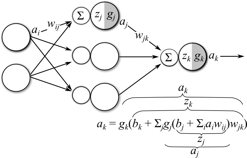
Figure 1: Diagram of an artificial neural network with a single hidden layer (bias units not shown)

---

Training a neural network involves determining the set of parameters $\mathbf{\theta} = \{\mathbf{W},\mathbf{b}\}$ that reduces the amount errors that the network makes. Often the choice for the error function is the sum of the squared errors between the target values $t_k$ and the network output $a_k$:

$$\begin{align} E &= \frac{1}{2} \sum_{k=1}^K(a_k - t_k)^2 \tag{1} \end{align}$$

Where $K$ is the dimensionality of the target/output for a single observation. This parameter optimization problem can be solved using gradient descent, which requires determining $\frac{\partial E}{\partial \theta}$ for all $\theta$ in the model.

Before we begin, let’s define the notation that will be used in remainder of the derivation. Please refer to Figure 1 for any clarifications.

• ${z_j}$: input to node $j$ in layer $l$
• ${g_j}$: activation function for node $j$ in layer $l$ (applied to ${z_j}$)
• $a_j=g_j(z_j)$: the output/activation of node $j$ in layer $l$
• ${b_{j}}$: bias/offset for unit $j$ in layer $l$
• ${w_{ij}}$: weights connecting node $i$ in layer $(l-1)$ to node $j$ in layer $l$
• ${t_{k}}$: target value for node $k$ in the output layer

Also note that the parameters for an ANN can be broken up into two distinct sets: those parameters that are associated with the output layer (i.e. $\theta_k = \{w_{jk}, b_k\}$), and thus directly affect the network output error; and the remaining parameters that are associated with the hidden layer(s), and thus affect the output error indirectly. We’ll first derive the gradients for the output layer parameters, then extend these results to the hidden layer parameters.

Gradients for Output Layer Parameters

Output layer connection weights, $w_{jk}$

Since the output layer parameters directly affect the value of the error function, determining the gradient of the error function with respect to those parameters is fairly straight-forward using an application of the chain rule²:

$$\begin{align} \frac{\partial E }{\partial w_{jk}} &= \frac{1}{2} \sum_{k}(a_k - t_k)^2 \\ &= (a_k - t_k)\frac{\partial}{\partial w_{jk}}(a_k - t_k) \tag{2} \end{align}$$

The derivative with respect to $t_k$ is zero because it does not depend on $w_{jk}$. We can also use the fact that $a_k = g(z_k)$, and re-apply the chain rule to give

$\begin{align}\frac{\partial E }{\partial w_{jk}} &= (a_k - t_k)\frac{\partial}{\partial w_{jk}}a_k \\ &= (a_k - t_k)\frac{\partial}{\partial w_{jk}}g_k(z_k) \\ &= (a_k - t_k)g_k'(z_k)\frac{\partial}{\partial w_{jk}}z_k \tag{3} \end{align}$.

Now, recall that $z_k = b_k + \sum_j g_j(z_j)w_{jk}$ and thus $\frac{\partial z_{k}}{\partial w_{jk}} = g_j(z_j) = a_j$, thus giving us:

$$\begin{align} \frac{\partial E }{\partial w_{jk}} &= \color{red}{(a_k - t_k)}\color{blue}{g_k'(z_k)}\color{green}{a_j} \end{align} \tag{4}$$

From *Equation 4 we can see that the gradient of the error function with respect to the output layer weights $w_{jk}$ is a product of three terms:

• $\color{red}{(a_k - t_k)}$: the difference between the network output $a_k$ and the target value $t_k$.
• $\color{blue}{g_k'(z_k)}$: the derivative of output layer activation function $g_k()$. For more details on activation function derivatives, please refer to this post
• $\color{green}{a_j}$: the activation signal of node $j$ from the hidden layer feeding into the output layer.

If we define $\delta_k$ to be all the terms that involve index $k$:

$$\color{purple}{\delta_k} = \color{red}{(a_k - t_k)}\color{blue}{g_k'(z_k)} \tag{5}$$

Then we get the “delta form” of the error function gradient for the output layer weights:

$$\frac{\partial E }{\partial w_{jk}} = \color{purple}{\delta_k} \color{green}{a_j} \tag{6}$$

Here the $\delta_k$ terms can be interpreted as the network output error after being “backpropagated” through the output activation function $g_k$, thus creating an “error signal”. Loosely speaking, Equation 6 can be interpreted as determining how much each $w_{jk}$ contributes to the error signal by weighting the error by the magnitude of the output activation from the previous (hidden) layer. The gradients with respect to each $w_{jk}$ are thus considered to be the “contribution” of that parameter to the total error signal and should be “negated” during learning. This gives the following gradient descent update rule for the output layer weights:

$$\begin{align} w_{jk} &\leftarrow w_{jk} - \eta \frac{\partial E }{\partial w_{jk}} \\ &\leftarrow w_{jk} - \eta (\color{purple}{\delta_k} \color{green}{a_j}) \tag{7} \end{align}$$

where $\eta$ is some step size, often referred to as the “learning rate”. Similar update rules are used to update the remaining parameters, once $\frac{\partial E}{\partial \theta}$ has been determined.

As we’ll see shortly, the process of “backpropagating” the error signal can repeated all the way back to the input layer by successively projecting $\delta_k$ back through $w_{jk}$, then through the activation function $g'_j(z_j)$ for the hidden layer to give the error signal $\delta_j$, and so on. This backpropagation concept is central to training neural networks with more than one layer.

Output layer biases, $b_{k}$

As for the gradient of the error function with respect to the output layer biases, we follow the same routine as above for $w_{jk}$. However, the third term in Equation 3 is $\frac{\partial}{\partial b_k} z_k = \frac{\partial}{\partial b_k} \left[ b_k + \sum_j g_j(z_j)\right] = 1$, giving the following gradient for the output biases:

$$\begin{align} \frac{\partial E }{\partial b_k} &= (a_k - t_k)g_k'(z_k)(1) \\ &= \color{purple}{\delta_k} \tag{8} \end{align}$$

Thus the gradient for the biases is simply the back-propagated error signal $\delta_k$ from the output units. One interpretation of this is that the biases are weights on activations that are always equal to one, regardless of the feed-forward signal. Thus the bias gradients aren’t affected by the feed-forward signal, only by the error.

Gradients for Hidden Layer Parameters

Now that we’ve derived the gradients for the output layer parameters and established the notion of backpropagation, let’s continue with this information in hand in order to derive the gradients for the remaining layers.

Hidden layer connection weights, $w_{ij}$

Due to the indirect affect of the hidden layer on the output error, calculating the gradients for the hidden layer weights $w_{ij}$ is somewhat more involved. However, the process starts just the same as for the output layer ³:

$$\begin{align} \frac{\partial E }{\partial w_{ij}} &= \frac{1}{2} \sum_{k}(a_k - t_k)^2 \\ &= \sum_{k} (a_k - t_k) \frac{\partial}{\partial w_{ij}}a_k \tag{9} \end{align}$$

Continuing on, noting that $a_k = g_k(z_k)$ and again applying chain rule, we obtain:

$$\begin{align} \frac{\partial E }{\partial w_{ij}} &= \sum_{k} (a_k - t_k) \frac{\partial }{\partial w_{ij}}g_k(z_k) \\ &= \sum_{k} (a_k - t_k)g'_k(z_k)\frac{\partial }{\partial w_{ij}}z_k \tag{10} \end{align}$$

Ok, now here’s where things get slightly more involved. Notice that the partial derivative $\frac{\partial }{\partial w_{ij}}z_k$ in Equation 10 is with respect to $w_{ij}$, but the target $z_k$ is a function of index $k$. How the heck do we deal with that!? If we expand $z_k$ a little, we find that it is composed of other sub functions:

$$\begin{align} z_k &= b_k + \sum_j a_jw_{jk} \\ &= b_k + \sum_j g_j(z_j)w_{jk} \\ &= b_k + \sum_j g_j(b_i + \sum_i a_i w_{ij})w_{jk} \tag{11} \end{align}$$

From Equation 11 we see that $z_k$ is indirectly dependent on $w_{ij}$. Equation 10 also suggests that we can again use the chain rule to calculate $\frac{\partial z_k }{\partial w_{ij}}$. This is probably the trickiest part of the derivation, and also requires noting that $z_j = b_j + \sum_i a_iw_{ij}$ and $a_j=g_j(z_j)$:

$$\begin{align} \frac{\partial z_k }{\partial w_{ij}} &= \frac{\partial z_k}{\partial a_j}\frac{\partial a_j}{\partial w_{ij}} \\ &= \frac{\partial}{\partial a_j} (b_k + \sum_j a_jw_{jk}) \frac{\partial a_j}{\partial w_{ij}} \\ &= w_{jk}\frac{\partial a_j}{\partial w_{ij}} \\ &= w_{jk}\frac{\partial g_j(z_j)}{\partial w_{ij}} \\ &= w_{jk}g_j'(z_j)\frac{\partial z_j}{\partial w_{ij}} \\ &= w_{jk}g_j'(z_j)\frac{\partial}{\partial w_{ij}}(b_j + \sum_i a_i w_{ij}) \\ &= w_{jk}g_j'(z_j)a_i \tag{12} \end{align}$$

Now, plugging Equation 12 into $\frac{\partial z_k}{\partial w_{ij}}$ into Equation 10 gives the following expression for $\frac{\partial E}{\partial w_{ij}}$:

$$\begin{align} \frac{\partial E }{\partial w_{ij}} &= \sum_{k} (a_k - t_k)g'_k(z_k)w_{jk} g'_j(z_j)a_i \\ &= \left(\sum_{k} \color{purple}{\delta_k} w_{jk} \right) \color{darkblue}{g'_j(z_j)}\color{darkgreen}{a_i} \tag{13} \end{align}$$

Notice that the gradient for the hidden layer weights has a similar form to that of the gradient for the output layer weights. Namely the gradient is composed of three terms:

• the current layer’s activation function $\color{darkblue}{g'_j(z_j)}$
• the output activation signal from the layer below $\color{darkgreen}{a_i}$.
• an error term $\sum_{k} \color{purple}{\delta_k} w_{jk}$

For the output layer weight gradients, the error term was simply the difference in the target and output layer activations $\color{red}{a_k - t_k}$. Here, the error term includes not only the output layer error signal, $\delta_k$, but this error signal is further projected onto $w_{jk}$. Analogous to the output layer weights, the gradient for the hidden layer weights can be interpreted as a proxy for the “contribution” of the weights to the output error signal. However, for hidden layers, this error can only be “observed” from the point-of-view of the weights by backpropagating the error signal through the layers above the hidden layer.

To make this idea more explicit, we can define the resulting error signal backpropagated to layer $j$ as $\delta_j$, which includes all terms in Equation 13 that involve index $j$. This definition results in the following gradient for the hidden unit weights:

$$\color{darkred}{\delta_j} = \color{darkblue}{g'_j(z_j)} \sum_{k} \color{purple}{\delta_k} w_{jk} \tag{14}$$

Thus giving the final expression for the gradient:

$$\frac{\partial E }{\partial w_{ij}} = \color{darkred}{\delta_j}\color{darkgreen}{a_i} \tag{15}$$

Equation 15 suggests that in order to calculate the weight gradients at any layer $l$ in an arbitrarily-deep neural network, we simply need to calculate the backpropagated error signal $\delta_l$ that reaches that layer from the “above” layers, and weight it by the feed-forward signal $a_{l-1}$ feeding into that layer.

Hidden Layer Biases, $b_j$

Calculating the error gradients with respect to the hidden layer biases $b_j$ follows a very similar procedure to that for the hidden layer weights where, as in Equation 12, we use the chain rule to calculate $\frac{\partial z_k}{\partial b_j}$.

$$\begin{align} \frac{\partial E }{\partial b_{j}} &= \sum_{k} (a_k - t_k) \frac{\partial }{\partial b_{j}}g_k(z_k) \\ &= \sum_{k} (a_k - t_k)g'_k(z_k)\frac{\partial z_k}{\partial b_{j}} \tag{16} \end{align}$$

Again, using the chain rule to solve for $\frac{\partial z_k }{\partial b_{j}}$

$$\begin{align} \frac{\partial z_k }{\partial b_{j}} &= \frac{\partial z_k}{\partial a_j}\frac{\partial a_j}{\partial b_{j}} \\ &= \frac{\partial}{\partial a_j}(b_k + \sum_j a_j w_{jk})\frac{\partial a_j}{\partial b_{j}} \\ &= w_{jk}\frac{\partial a_j}{\partial b_{j}} \\ &= w_{jk}\frac{\partial g_j(z_j)}{\partial b_{j}} \\ &= w_{jk}g_j'(z_j)\frac{\partial z_j}{\partial b_{j}} \\ &= w_{jk}g_j'(z_j)\frac{\partial}{\partial b_j}(b_j + \sum_i a_i w_{ij}) \\ &= w_{jk}g_j'(z_j)(1) \tag{17} \end{align}$$

Plugging Equation 17 into the expression for $\frac{\partial z_k }{\partial b_j}$ in Equation 16 gives the final expression for the hidden layer bias gradients:

$$\begin{align} \frac{\partial E }{\partial b_j} &= \sum_{k} (a_k - t_k)g'_k(z_k) w_{jk} g_j'(z_j) \\ &= g'_j(z_j) \sum_{k} \delta_k w_{jk} \\ &= \color{darkred}{\delta_j} \tag{18} \end{align}$$

In a similar fashion to calculation of the bias gradients for the output layer, the gradients for the hidden layer biases are simply the backpropagated error signal reaching that layer. This suggests that we can also calculate the bias gradients at any layer $l$ in an arbitrarily-deep network by simply calculating the backpropagated error signal reaching that layer $\delta_l$. Pretty cool!

Wrapping up

In this post we went over some of the formal details of the backpropagation learning algorithm. The math covered in this post allows us to train arbitrarily deep neural networks by re-applying the same basic computations. In a later post, we’ll go a bit deeper in implementation and applications of neural networks, referencing this post for the formal development of the underlying calculus required for gradient descent.

---

---

Notes

1. Though, I guess these days with autograd, who really needs to understand how the calculus for gradient descent works, amiright? (hint: that is a joke) ↩

2. You may also notice that the summation disappears in the derivative. This is because when we take the partial derivative with respect to the $j$-th dimension/node. Therefore the only term that survives in the error gradient is the $j$-th, and we can thus ignore the remaining terms in the summation. ↩

3. Notice here that the sum does not disappear in the derivative as it did for the output layer parameters. This is due to the fact that the hidden layers are fully connected, and thus each of the hidden unit outputs affects the state of each output unit. ↩